Data Engineering Project for Beginners - Batch edition
- 1. Introduction
- 2. Objective
- 3. Design
- 4. Setup
- 5. Code walkthrough
- 6. Tear down infra
- 7. Design considerations
- 8. Next steps
- 9. Conclusion
- 10. Further reading
- 11. References
1. Introduction
A real data engineering project usually involves multiple components. Setting up a data engineering project, while conforming to best practices can be extremely time-consuming. If you are
A data analyst, student, scientist, or engineer looking to gain data engineering experience, but are unable to find a good starter project.
Wanting to work on a data engineering project that simulates a real-life project.
Looking for an end-to-end data engineering project.
Looking for a good project to get data engineering experience for job interviews.
Then this tutorial is for you. In this tutorial, you will
-
Set up Apache Airflow, AWS EMR, AWS Redshift, AWS Spectrum, and AWS S3.
-
Learn data pipeline best practices.
-
Learn how to spot failure points in data pipelines and build systems resistant to failures.
-
Learn how to design and build a data pipeline from business requirements.
If you are interested in a stream processing project, please check out Data Engineering Project for Beginners - Stream Edition . If you are interested in a local only data engineering project, checkout this post .
2. Objective
Let’s assume that you work for a user behavior analytics company that collects user data and creates a user profile. We are tasked with building a data pipeline to populate the user_behavior_metric table. The user_behavior_metric table is an OLAP table, meant to be used by analysts, dashboard software, etc. It is built from
user_purchase: OLTP table with user purchase information.movie_review.csv: Data sent every day by an external data vendor.
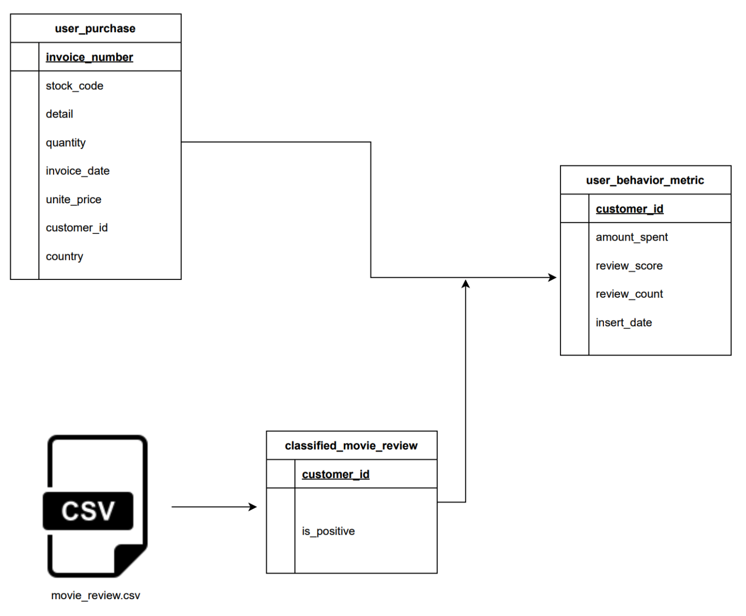
3. Design
We will be using Airflow to orchestrate the following tasks:
- Classifying movie reviews with Apache Spark.
- Loading the classified movie reviews into the data warehouse.
- Extracting user purchase data from an OLTP database and loading it into the data warehouse.
- Joining the classified movie review data and user purchase data to get
user behavior metricdata.
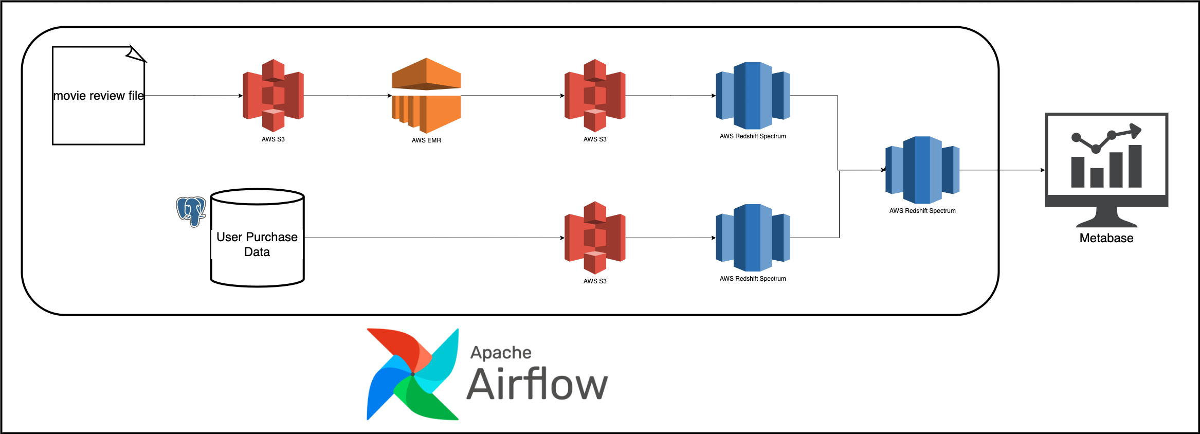
We will use metabase to visualize our data.
4. Setup
4.1 Prerequisite
- git
- Github account
- Terraform
- AWS account
- AWS CLI installed and configured
- Docker with at least 4GB of RAM and Docker Compose v1.27.0 or later
- psql
Read this post , for information on setting up CI/CD, DB migrations, IAC(terraform), “make” commands and automated testing.
Run these commands to setup your project locally and on the cloud.
# Clone and cd into the project directory.
git clone https://github.com/josephmachado/beginner_de_project.git
cd beginner_de_project

# Local run & test
make up # start the docker containers on your computer & runs migrations under ./migrations
make ci # Runs auto formatting, lint checks, & all the test files under ./tests

# Create AWS services with Terraform
make tf-init # Only needed on your first terraform run (or if you add new providers)
make infra-up # type in yes after verifying the changes TF will make

# Create Redshift Spectrum tables (tables with data in S3)
make spectrum-migration
# Create Redshift tables
make redshift-migration

# Wait until the EC2 instance is initialized, you can check this via your AWS UI
# See "Status Check" on the EC2 console, it should be "2/2 checks passed" before proceeding
# Wait another 5 mins, Airflow takes a while to start up

make cloud-airflow # this command will forward Airflow port from EC2 to your machine and opens it in the browser
# the user name and password are both airflow

make cloud-metabase # this command will forward Metabase port from EC2 to your machine and opens it in the browser
To get Redshift connection credentials for metabase use these commands.
make infra-config
# use redshift_dns_name as host
# use redshift_user & redshift_password
# dev as database
Since we cannot replicate AWS components locally, we have not set them up here. To learn more about how to set up components locally read this article
Create database migrations as shown below.
make db-migration # enter a description, e.g., create some schema
# make your changes to the newly created file under ./migrations
make redshift-migration # to run the new migration on your warehouse
For the continuous delivery
to work, set up the infrastructure with terraform, & defined the following repository secrets. You can set up the repository secrets by going to Settings > Secrets > Actions > New repository secret.
SERVER_SSH_KEY: We can get this by runningterraform -chdir=./terraform output -raw private_keyin the project directory and paste the entire content in a new Action secret called SERVER_SSH_KEY.REMOTE_HOST: Get this by runningterraform -chdir=./terraform output -raw ec2_public_dnsin the project directory.REMOTE_USER: The value for this is ubuntu.
We have a dag validity test defined here .
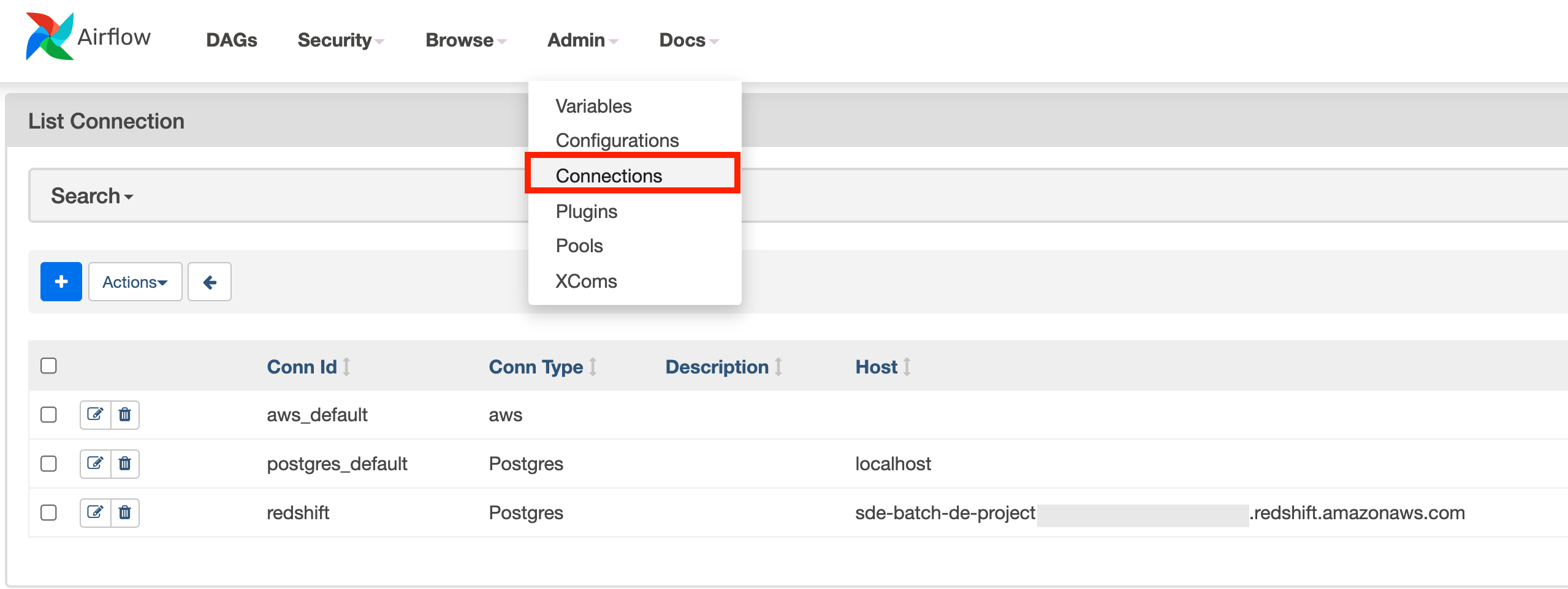
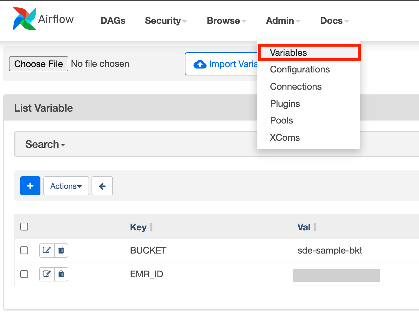
The make infra-up also creates Airflow connections and variables
.
redshift connection: To connect to the AWS Redshift cluster.postgres_default connection: To connect to the local Postgres database.BUCKET variable: To indicate the bucket to be used as the data lake for this pipeline.EMR_ID variable: To send commands to an AWS EMR cluster.
You can see them on Airflow’s UI as shown below.
4.2 AWS Infrastructure costs
We use
- 3
m4.xlargetype nodes for our AWS EMR cluster. - 1
dc2.largefor our AWS Redshift cluster. - 1
iam roleto allow Redshift access to S3. - 1
S3 bucketwith about 150MB in size. - 1
t2.largeAWS EC2 instance.
A very rough estimate would be 358.89 USD per month for our setup. This means our infrastructure will cost approximately about 0.49 USD per hour. Use this AWS cost calculator
to verify costs.
4.3 Data lake structure
We will use AWS S3 as our data lake. Data from external systems will be stored here for further processing. AWS S3 will be used as storage for use with AWS Redshift Spectrum.
In our project, we will use one bucket with multiple folders.
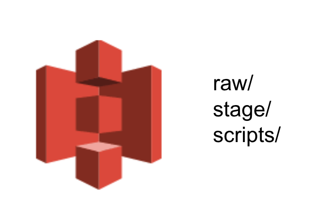
- raw: To store raw data. This is denoted as
Raw Areain the design section. - stage: This is denoted as
Stage Areain the design section. - scripts: This is used to store spark script, for use by AWS EMR.
This pattern will let us create different buckets for different environments.
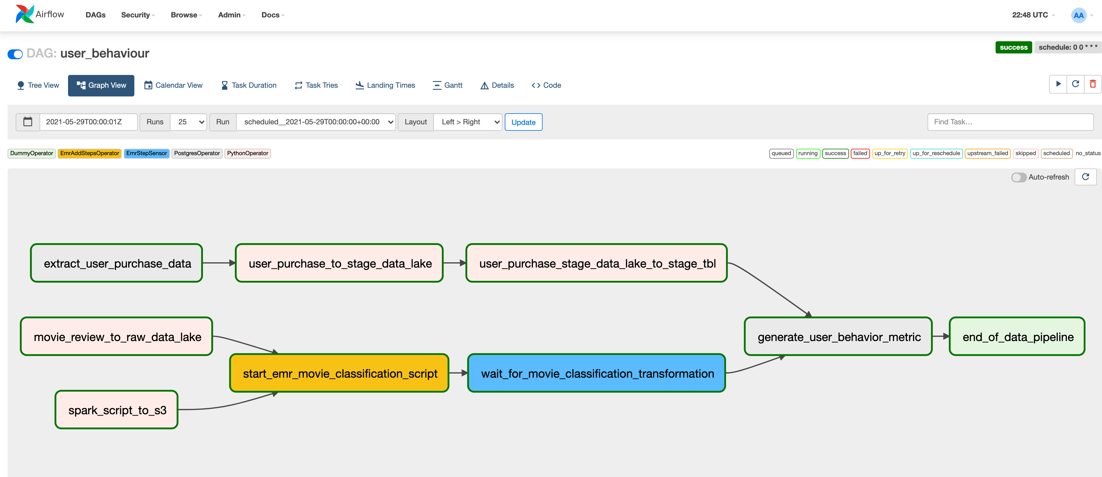
5. Code walkthrough
The data for user_behavior_metric is generated from 2 main datasets. We will look at how each of them is ingested, transformed, and used to get the data for the final table.
5.1 Loading user purchase data into the data warehouse
To load the user purchase data from Postgres into AWS Redshift we run the following tasks.
- extract_user_purchase_data: Unloads data from Postgres to a local file system in the Postgres container. This filesystem is volume synced between our local Postgres and Airflow containers. This allows Airflow to access this data.
- user_purchase_to_stage_data_lake: Moves the extracted data to data lake’s staging area at
stage/user_purchase/{{ ds }}/user_purchase.csv, wheredswill be replaced by the run date inYYYY-MM-DDformat. Thisdswill serve as theinsert_datepartition, defined at table creation. - user_purchase_stage_data_lake_to_stage_tbl: Runs a Redshift query to make the
spectrum.user_purchase_stagingtable aware of the new date partition.

extract_user_purchase_data = PostgresOperator(
    dag=dag,
    task_id="extract_user_purchase_data",
    sql="./scripts/sql/unload_user_purchase.sql",
    postgres_conn_id="postgres_default",
    params={"user_purchase": "/temp/user_purchase.csv"},
    depends_on_past=True,
    wait_for_downstream=True,
)

user_purchase_to_stage_data_lake = PythonOperator(
    dag=dag,
    task_id="user_purchase_to_stage_data_lake",
    python_callable=_local_to_s3,
    op_kwargs={
        "file_name": "/temp/user_purchase.csv",
        "key": "stage/user_purchase/{{ ds }}/user_purchase.csv",
        "bucket_name": BUCKET_NAME,
        "remove_local": "true",
    },
)

user_purchase_stage_data_lake_to_stage_tbl = PythonOperator(
    dag=dag,
    task_id="user_purchase_stage_data_lake_to_stage_tbl",
    python_callable=run_redshift_external_query,
    op_kwargs={
        "qry": "alter table spectrum.user_purchase_staging add if not exists partition(insert_date='{{ ds }}') \
            location 's3://"
        + BUCKET_NAME
        + "/stage/user_purchase/{{ ds }}'",
    },
)

extract_user_purchase_data >> user_purchase_to_stage_data_lake >> user_purchase_stage_data_lake_to_stage_tbl
./scripts/sql/unload_user_purchase.sql
COPY (
       select invoice_number,
              stock_code,
              detail,
              quantity,
              invoice_date,
              unit_price,
              customer_id,
              country
       from retail.user_purchase -- we should have a date filter here to pull only required date's data
) TO '{{ params.user_purchase }}' WITH (FORMAT CSV, HEADER);
-- user_purchase will be replaced with /temp/user_purchase.csv from the params in extract_user_purchase_data task
It’s not always a good pattern to store the entire dataset in our local filesystem. Since we could get an out-of-memory error if our dataset is too large. So, an alternative would be to have a streaming process that writes in batches to our data lake, as shown here .
5.2 Loading classified movie review data into the data warehouse
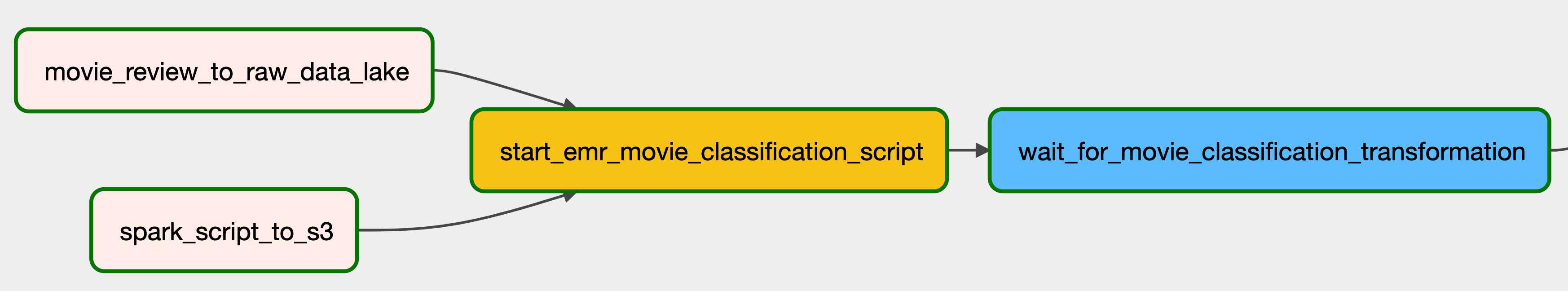
To get the classified movie review data into AWS Redshift, we run the following tasks:
- movie_review_to_raw_data_lake: Copies local file
data/movie_review.csvto data lake’s raw area. - spark_script_to_s3: Copies our pyspark script to data lake’s script area. This allows AWS EMR to reference it.
- start_emr_movie_classification_script: Adds the EMR steps
defined at
dags/scripts/emr/clean_movie_review.jsonto our EMR cluster. This task adds 3 EMR steps to the cluster, they do the following- Moves raw data from S3 to HDFS: Copies data from data lake’s raw area into EMR’s HDFS.
- Classifies movie reviews: Runs the review classification pyspark script.
- Moves classified data from HDFS to S3: Copies data from EMR’s HDFS to data lake’s staging area.
- wait_for_movie_classification_transformation: This is a sensor task that waits for the final step (
Move classified data from HDFS to S3) to finish.
movie_review_to_raw_data_lake = PythonOperator(
    dag=dag,
    task_id="movie_review_to_raw_data_lake",
    python_callable=_local_to_s3,
    op_kwargs={
        "file_name": "/data/movie_review.csv",
        "key": "raw/movie_review/{{ ds }}/movie.csv",
        "bucket_name": BUCKET_NAME,
    },
)

spark_script_to_s3 = PythonOperator(
    dag=dag,
    task_id="spark_script_to_s3",
    python_callable=_local_to_s3,
    op_kwargs={
        "file_name": "./dags/scripts/spark/random_text_classification.py",
        "key": "scripts/random_text_classification.py",
        "bucket_name": BUCKET_NAME,
    },
)

start_emr_movie_classification_script = EmrAddStepsOperator(
    dag=dag,
    task_id="start_emr_movie_classification_script",
    job_flow_id=EMR_ID,
    aws_conn_id="aws_default",
    steps=EMR_STEPS,
    params={
        "BUCKET_NAME": BUCKET_NAME,
        "raw_movie_review": "raw/movie_review",
        "text_classifier_script": "scripts/random_text_classifier.py",
        "stage_movie_review": "stage/movie_review",
    },
    depends_on_past=True,
)

last_step = len(EMR_STEPS) - 1

wait_for_movie_classification_transformation = EmrStepSensor(
    dag=dag,
    task_id="wait_for_movie_classification_transformation",
    job_flow_id=EMR_ID,
    step_id='{{ task_instance.xcom_pull("start_emr_movie_classification_script", key="return_value")['
    + str(last_step)
    + "] }}",
    depends_on_past=True,
)

[
    movie_review_to_raw_data_lake,
    spark_script_to_s3,
] >> start_emr_movie_classification_script >> wait_for_movie_classification_transformation
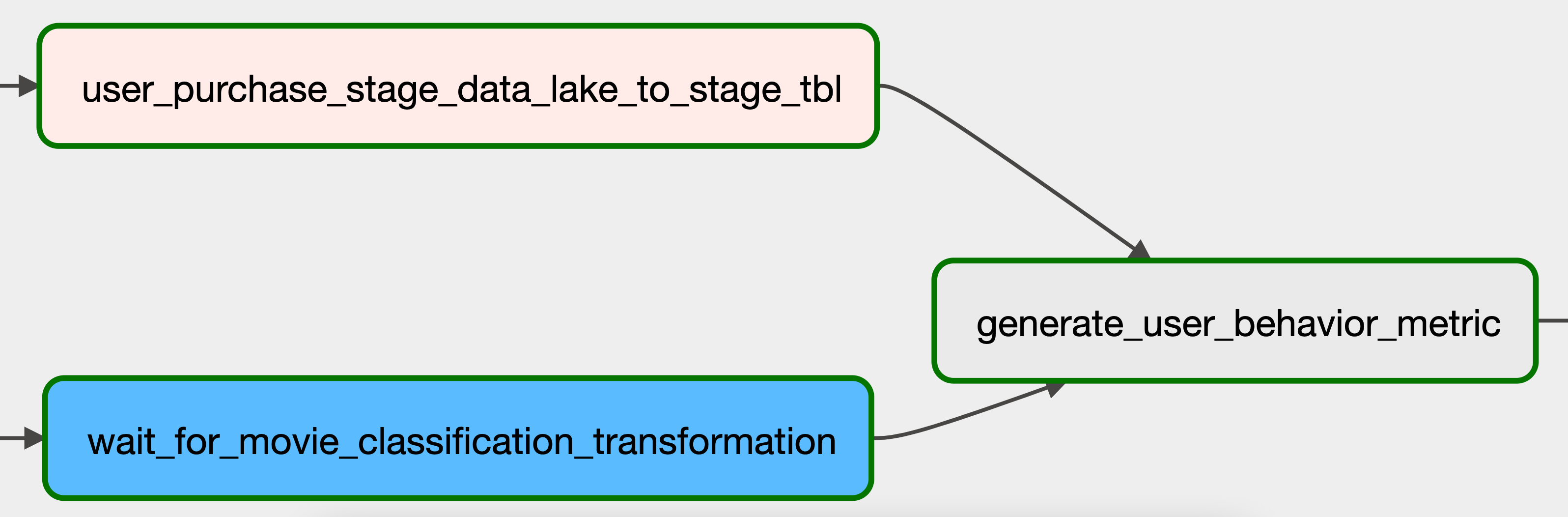
5.3 Generating user behavior metric
With both the user purchase data and the classified movie data in the data warehouse, we can get the data for the user_behavior_metric table. This is done using the generate_user_behavior_metric task. This task runs a redshift SQL script to populate the public.user_behavior_metric table.
generate_user_behavior_metric = PostgresOperator(
    dag=dag,
    task_id="generate_user_behavior_metric",
    sql="scripts/sql/generate_user_behavior_metric.sql",
    postgres_conn_id="redshift",
)

end_of_data_pipeline = DummyOperator(task_id="end_of_data_pipeline", dag=dag) # dummy operator to indicate DAG complete

[
    user_purchase_stage_data_lake_to_stage_tbl,
    wait_for_movie_classification_transformation,
] >> generate_user_behavior_metric >> end_of_data_pipeline
The sql query generates customer level aggregate metrics, using spectrum.user_purchase_staging and spectrum.classified_movie_review.
-- scripts/sql/generate_user_behavior_metric.sql

DELETE FROM public.user_behavior_metric
WHERE insert_date = '{{ ds }}';
INSERT INTO public.user_behavior_metric (
        customerid,
        amount_spent,
        review_score,
        review_count,
        insert_date
    )
SELECT ups.customerid,
    CAST(
        SUM(ups.Quantity * ups.UnitPrice) AS DECIMAL(18, 5)
    ) AS amount_spent,
    SUM(mrcs.positive_review) AS review_score,
    count(mrcs.cid) AS review_count,
    '{{ ds }}'
FROM spectrum.user_purchase_staging ups
    JOIN (
        SELECT cid,
            CASE
                WHEN positive_review IS True THEN 1
                ELSE 0
            END AS positive_review
        FROM spectrum.classified_movie_review
        WHERE insert_date = '{{ ds }}'
    ) mrcs ON ups.customerid = mrcs.cid
WHERE ups.insert_date = '{{ ds }}'
GROUP BY ups.customerid;
Log on to www.localhost:8080
to see the Airflow UI. The username and password are both airflow. Turn on the DAG. It can take about 10min to complete one run.
5.4. Checking results
You can check the public.user_behavior_metric redshift table from your terminal as shown below.
export REDSHIFT_HOST=$(aws redshift describe-clusters --cluster-identifier sde-batch-de-project --query 'Clusters[0].Endpoint.Address' --output text)
psql postgres://sde_user:sdeP0ssword0987@$REDSHIFT_HOST:5439/dev
In the SQL prompt, use the following queries to see the generated data.
select insert_date, count(*) as cnt from spectrum.classified_movie_review group by insert_date order by cnt desc; -- 100,000 per day
select insert_date, count(*) as cnt from spectrum.user_purchase_staging group by insert_date order by cnt desc; -- 541,908 per day
select insert_date, count(*) as cnt from public.user_behavior_metric group by insert_date order by cnt desc; -- 908 per day
\q
You can also connect to Metabase running www.localhost:3000 and visualize the data, as shown below.
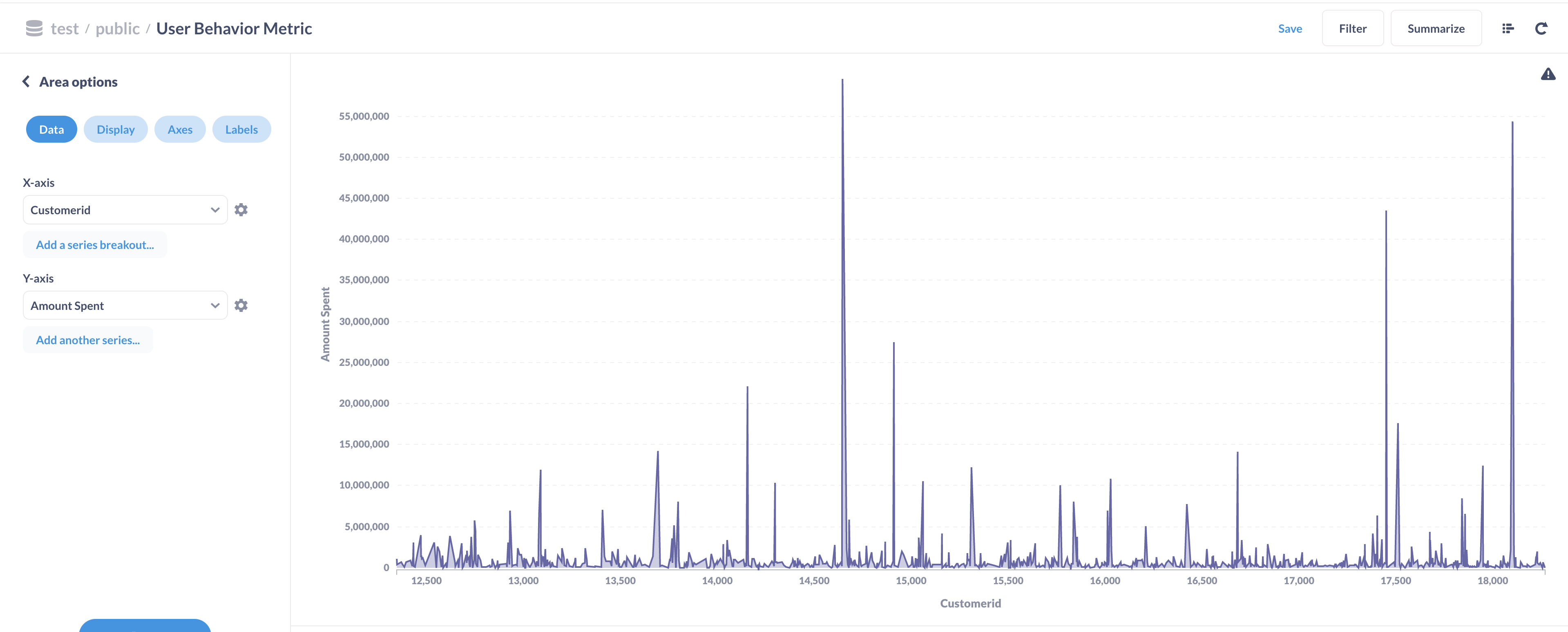
The counts should match.
6. Tear down infra
After you are done, make sure to destroy your cloud infrastructure.
make down # Stop docker containers on your computer
make infra-down # type in yes after verifying the changes TF will make
This will stop all the AWS services. Please double-check this by going to the AWS UI S3, EC2, EMR, & Redshift consoles.
7. Design considerations
Now that you have the data pipeline running successfully, it’s time to review some design choices.
-
Idempotent data pipeline
Check that all the tasks are idempotent. If you re-run a partially run or a failed task, your output should not be any different than if the task had run successfully. Read this article to understand idempotency in detail .
Hint, there is at least one non-idempotent task. -
Monitoring & Alerting
The data pipeline can be monitored from the Airflow UI. EMR Steps can be monitored via the AWS UI. We do not have any alerting in case of task failures, data quality issues, hanging tasks, etc. In real projects, there is usually a monitoring and alerting system. Some common systems used for monitoring and alerting are
cloud watch,datadog, ornewrelic. -
Quality control
We do not check for data quality in this data pipeline. We can set up basic count, standard deviation, etc checks before we load data into the final table. For advanced testing requirements consider using a data quality framework, such as great_expectations .
-
Concurrent runs
If you have to re-run the pipeline for the past 3 months, it would be ideal to have them run concurrently and not sequentially. We can set levels of concurrency as shown here . Even with an appropriate concurrency setting, our data pipeline has one task that is blocking. Figuring out the blocking task is left as an exercise for the reader.
-
Changing DAG frequency
What are the changes necessary to run this DAG every hour? How will the table schema need to change to support this? Do you have to rename the DAG?
-
Backfills
Assume you have a logic change in the movie classification script. You want this change to be applied to the past 3 weeks. If you want to re-run the data pipeline for the past 3 weeks, will you
re-run the entire DAG or only parts of it. Why would you choose one option over the other? You can use this command to run backfills. Prefix the command withdocker exec -d beginner_de_project_airflow-webserver_1to run it on our Airflow docker container. -
Data size
Will the data pipeline run successfully if your data size increases by 10x, 100x, 1000x why? why not?
8. Next steps
If you are interested in working more with this data pipeline, please consider contributing to the following.
- Unit tests, DAG run tests, and integration tests.
- Use Taskflow API for the DAG.
If you have other ideas, please feel free to open Github issues or pull requests .
9. Conclusion
Hope this article gives you a good idea of how to design and build an end-to-end data pipeline. To recap, we saw:
- Infrastructure setup
- Data pipeline best practices
- Design considerations
- Next steps
Please leave any questions or comments in the comment section below.
10. Further reading
- Airflow pros and cons
- What is a data warehouse
- What and why staging?
- Beginner DE project - Stream edition
- How to submit spark EMR jobs from Airflow
- DE project to impress hiring manager