3 Key techniques, to optimize your Apache Spark code

• Intro
• Distributed Systems
  • 1. Distributed storage systems
  • 2. Distributed data processing
    • Traditional data processing
    • Distributed data processing
• Setup
  • AWS Setup
• Optimizing your spark code
• Technique 1: reduce data shuffle
  • Spark UI
    • Spark History Server
    • Narrow Transformation
  • Key points
• Technique 2. Use caching, when necessary - Saving plateTypeCountDF without cache - Saving plateTypeAvgDF without cache - Saving plateTypeCountDF with cache - Saving plateTypeAvgDF with cache
  • user exercise
  • Key points
• Technique 3. Join strategies - broadcast join and bucketed joins
  • 3.1. Broadcast Join
  • 3.2. Bucketed Join
    • user exercise
    • Key points
• TL; DR
• Conclusion
  • Reference:

Intro

A lot of tutorials show how to write spark code with just the API and code samples, but they do not explain how to write “efficient Apache Spark” code. Some comments from users of Apache Spark

“The biggest challenge with spark is not in writing the transformations but making sure they can execute with big enough data sets”

“The issue isn’t the syntax or the methods, it’s figuring out why, when I do it this time does the execution take an hour when last time it was 2 minutes”

“big data and distributed systems can be hard”

In this tutorial you will learn 3 powerful techniques used to optimize Apache Spark code. There is no one size fits all solution for optimizing Spark, use the techniques discussed below to decide on the optimal strategy for your use case.

Distributed Systems

Before we look at techniques to optimize Apache Spark, we should understand what distributed systems are and how they work.

1. Distributed storage systems

What is a distributed storage system? Let’s assume we have a file which is 500 TB in size, most machines do not have the amount of disk space necessary to store this file. In such cases the idea is to connect a cluster of machines(aka nodes) together and split the 500 TB file into smaller (128MB by default in HDFS) chunks and spread it across the different nodes in the cluster.

For e.g. if we want to move our 500 TB file into a HDFS cluster, the steps that happen internally are

1. The 500 TB file in broken down into multiple chunks, default size of 128MB each.
2. These chunks are replicated twice, so we have 3 copies of the same data. The number of copies is called replication factor and by default is set to 3 to prevent data loss even if 2 nodes that contain the chunk copies fail.
3. Then they are moved into the nodes in the cluster.
4. The HDFS system makes sure the chunks are distributed amongst the nodes in the cluster such that even if a node containing some data fails, the data can be accessed from its replicas in other nodes.

The reason someone would want to use distributed storage is

1. Their data is too large to be stored in a single machine.
2. Their application are stateless and dumps all their data into a distributed storage.
3. They want to analyze large amounts of data.

2. Distributed data processing

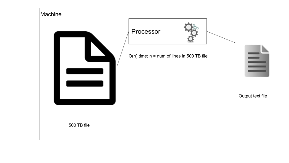
In traditional data processing you bring the data to the machine where you process it. In our case, let’s say we want to filter out certain rows from our 500 TB file, we can run a simple script that streams through the file one line at a time and based on the filter outputs some data.

Traditional data processing

Now your script has to process the data file one line at a time, but what if we can use a distributed storage system and process the file in parallel? This is the foundational idea behind distributed data processing. In order to process data that has been distributed across nodes we use distributed data processing systems. Most data warehouses such as Redshift, Big query, Hive, use this model to process the data. Let’s consider the same case where we have to filter our 500 TB data, but this time the data is in a distributed storage system. In this case we use a distributed data processing system such as Apache Spark, the main difference here is that the data processing logic is moved to the data location where the data is processed, this way we reduce moving large data around. In the below diagram you can see in node 1 the processing is done within the node and written out to disk of the same node.

Distributed data processing

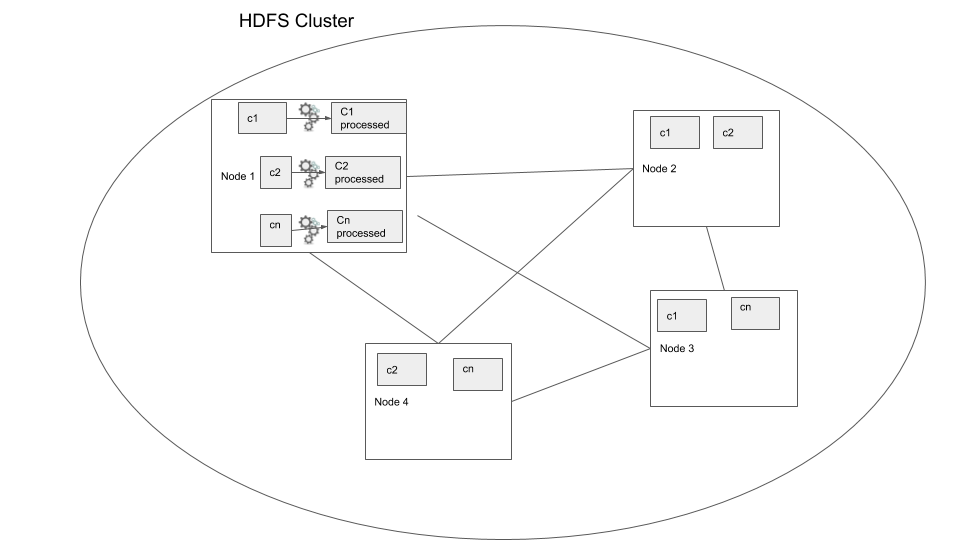
In the above example we can see how the process would be much faster because the process is being run in parallel. But this is a very simple example where we keep the data processing “local”, that is the data is not moved over the network. This is called a local transformation.

Now that we have a good understanding of what distributed data storage and processing is, we can start to look at some techniques to optimize Apache Spark code.

Setup

We are going to use AWS EMR to run a Spark, HDFS cluster.

AWS Setup

1. Create an AWS account
2. Create a pem file, follow the steps here
3. Start a EMR cluster, follow the steps here , make sure to note down you master’s public DNS
4. Move data into your EMR cluster using the steps shown below

SSH into your EMR master node

ssh -i ~/.ssh/sde.pem hadoop@<your-master-public-dns>
# master-public-dns sample: ec2-3-91-31-191.compute-1.amazonaws.com

The connection sometimes dies, so install tmux to be able to stay signed in

sudo yum install tmux -y
tmux new -s spark
wget https://www.dropbox.com/s/3uo4gznau7fn6kg/Archive.zip
unzip Archive.zip
hdfs dfs -ls / # list all the HDFS folder
hdfs dfs -mkdir /input # make a directory called input in HDFS
hdfs dfs -copyFromLocal  2015.csv /input # copy data from local Filesystem to HDFS
hdfs dfs -copyFromLocal  2016.csv /input
hdfs dfs -ls /input # check to see your copied data

wget https://www.dropbox.com/s/yuw9m5dbg03sad8/plate_type.csv
hdfs dfs -mkdir /mapping
hdfs dfs -copyFromLocal  plate_type.csv /mapping
hdfs dfs -ls /mapping

Now you have moved your data into HDFS and are ready to start working with it through Spark.

Optimizing your spark code

We will be using AWS EMR to run spark code snippets. A few things to know about spark before we start

1. Apache Spark is lazy loaded, ie it does not perform the operations until we require an output. eg: If we filter a data frame based on a certain field it does not get filtered immediately but only when you write the output to a file system or the driver requires some data. The advantage here is that Spark can actually optimize the execution based on the entire execution logic before starting to process the data. So if you perform some filtering, joins, etc and then finally write the end result to a file system, only then is the logic executed by Apache Spark.

2. Apache Spark is a distributed data processing system and open source.

In this post we will be working exclusively with dataframes, although we can work with RDDs, dataframes provide a nice tabular abstraction which makes processing data easier and is optimized automatically for us. There are cases where using RDD is beneficial, but RDD does not have the catalyst optimizer or Tungsten execution engine which are enabled by default when we use dataframes.

Technique 1: reduce data shuffle

The most expensive operation in a distributed system such as Apache Spark is a shuffle. It refers to the transfer of data between nodes, and is expensive because when dealing with large amounts of data we are looking at long wait times. Let’s look at an example, start Apache spark shell using pyspark --num-executors=2 command

pyspark --num-executors=2 # num-executors to specify how many executors this spark job requires

parkViolations = spark.read.option("header", True).csv("/input/")
plateTypeCountDF = parkViolations.groupBy("Plate Type").count()
plateTypeCountDF.explain() # used to show the plan before execution, in the UI we can only see executed commands

We can use explain to view the query plan that is going to be used to read and process the data. Here we see a shuffle denoted by Exchange. We aim to reduce shuffles, but there are cases where we have to shuffle the data. GroupBy is one of those transformations. Since this involves a shuffle this transformation is called a wide-transformation. Let’s make Spark actually execute the operation by writing the output to a HDFS location.

plateTypeCountDF.write.format("com.databricks.spark.csv").option("header", True).mode("overwrite").save("/output/plate_type_count")
exit()

Spark UI

You can view the execution of your transformation using the Spark UI. You can get to it as shown below. NOTE: spark UI maybe slow sometimes, give it a few minutes after execution to display the DAGs.

Spark History Server

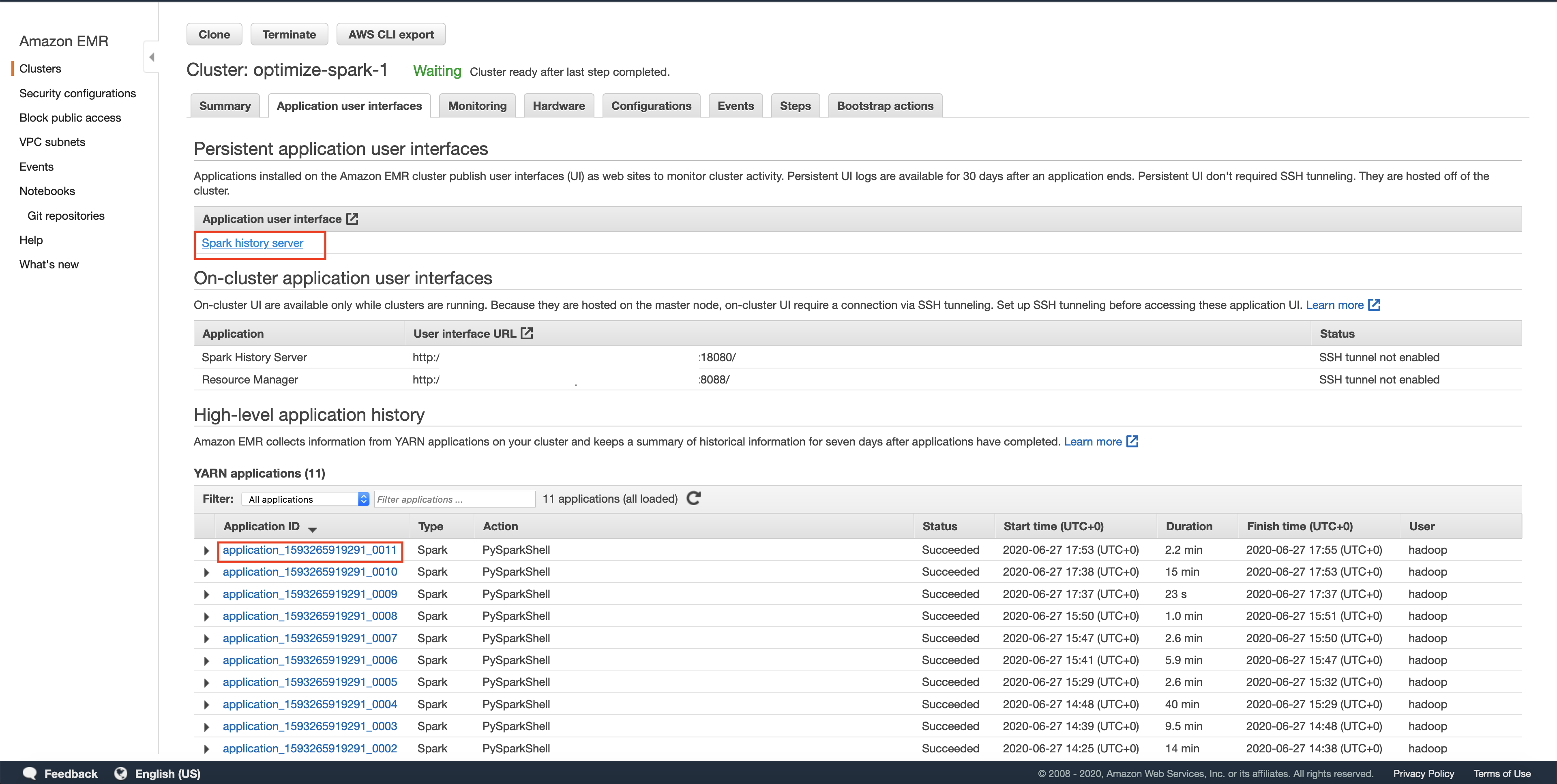
The history server will have a list of all the spark applications that have run. Sometimes you may have to wait for the application shown in AWS EMR UI to show up on the Spark UI, we can optimize this to be more real time, but since this is a toy example we leave it as such. In this post we will use a spark REPL(read-evaluate-print-loop) to try out the commands and exit after competing that section. Each spark REPL session corresponds to an application. Sometimes even after quitting the spark REPL, your application will still be in the Incomplete applications page.

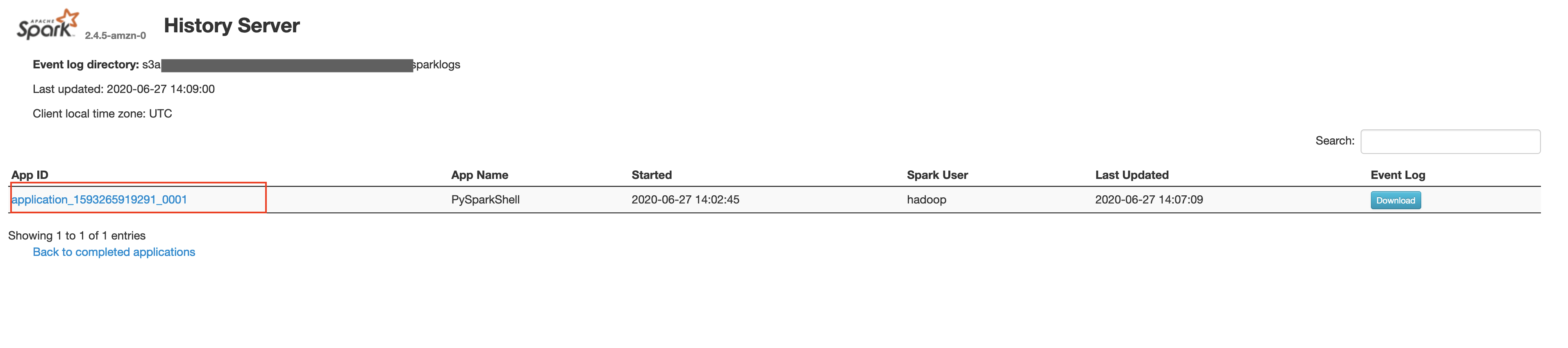
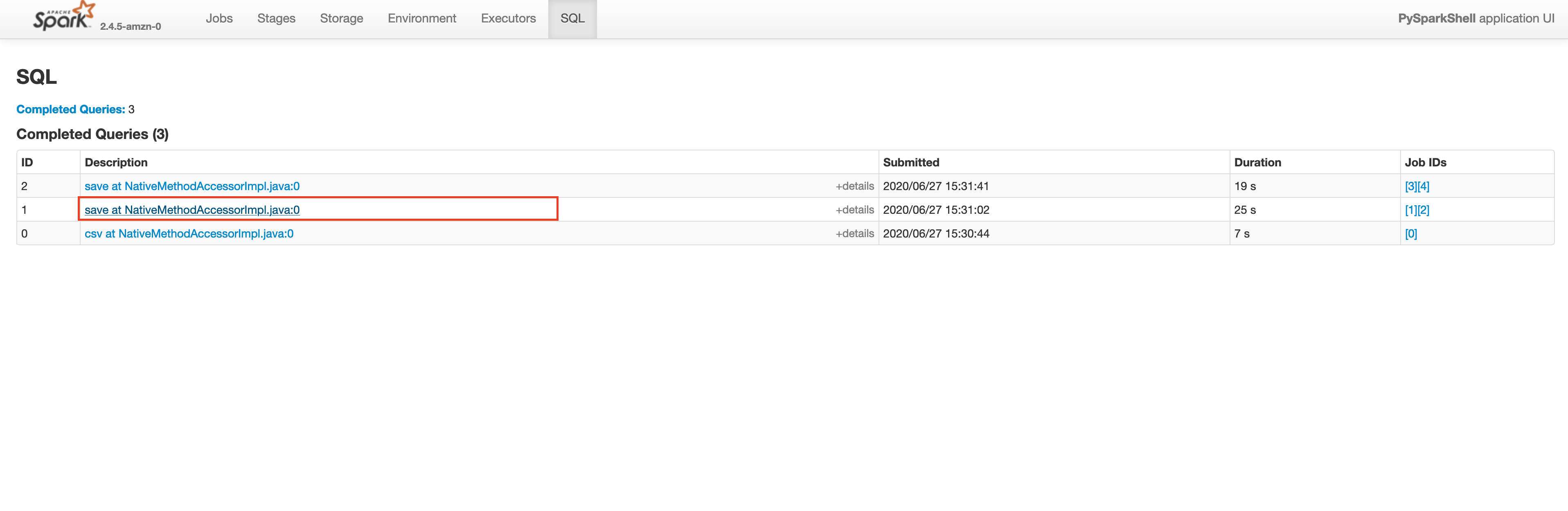
Make sure that the App ID you select in the spark history server is the latest one available in the AWS EMR's Application User Interface tab. Please wait for a few minutes if the application does not show up. This will take you to the lastest Apache Spark application. In the application level UI, you can see the individual transformations that have been executed. Go to the SQL tab and click on the save query, as shown below.

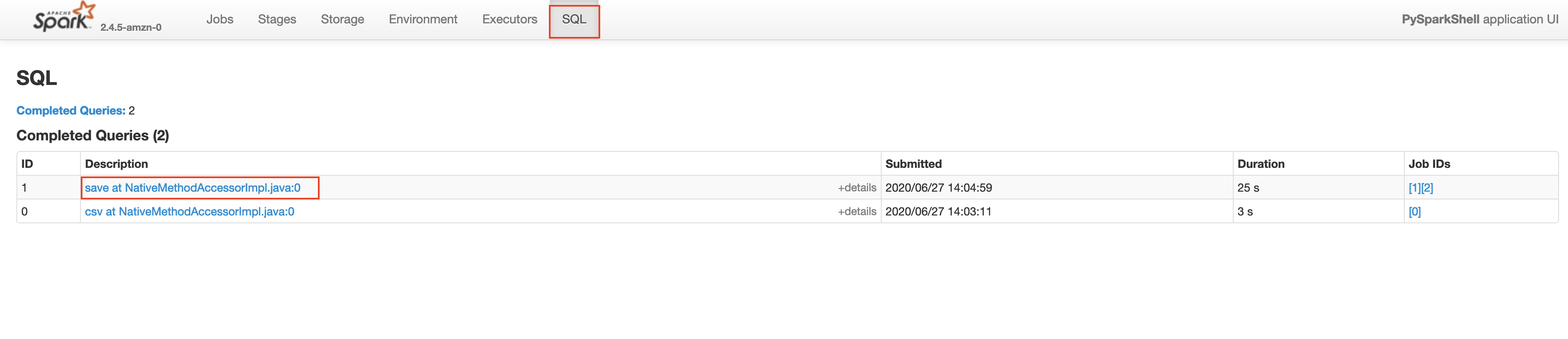
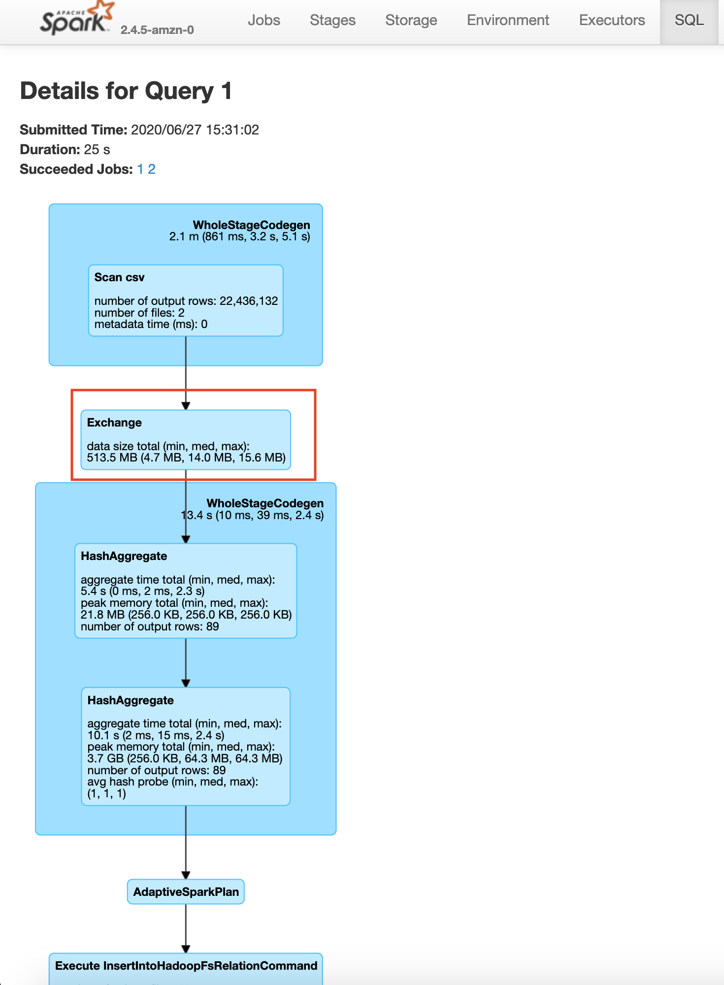
In the save query page, you will be able to see the exact process done by the Spark execution engine. You will notice a step in the process called exchange which is the expensive data shuffle process.

You can visualize the groupBy operation in a distributed cluster, as follows

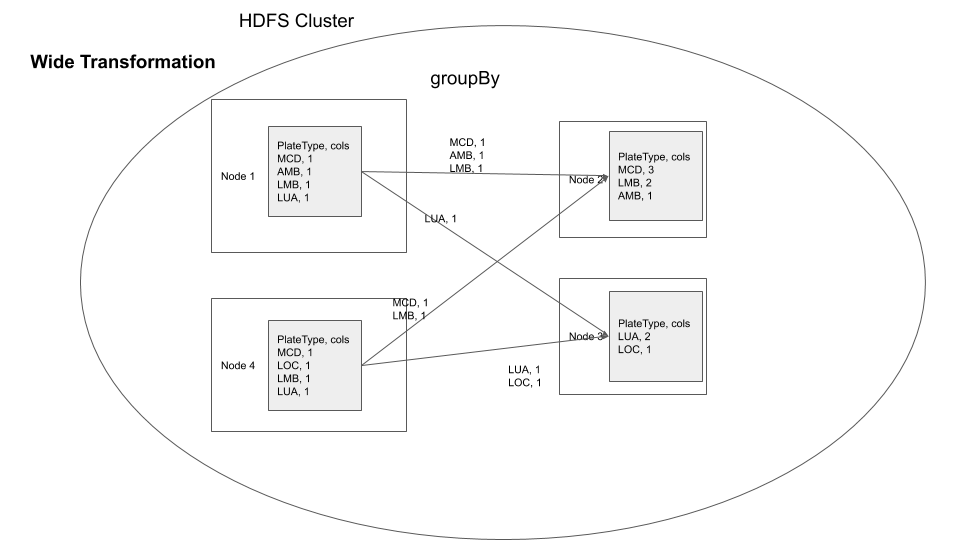
If you are performing groupBy multiple times on the same field, you can actually partition the data by that field and have subsequent groupBy transformations use that data. So what is partitioning, partitioning is a process where the data is split into multiple chunks based on a particular field or we can just specify the number of partitions . In our case, if we partition by the field Plate Type all the rows with similar Plate Type values end up in the same node. This means when we do groupBy there is no need for a data shuffle, thereby increasing the speed of the operation. This has the trade off that the data has to be partitioned first. As mentioned earlier use this technique. If you are performing groupBy multiple times on the same field multiple times or if you need fast query response time and are ok with preprocessing(in this case data shuffling ) the data.

pyspark --num-executors=2 # start pyspark shell

parkViolations = spark.read.option("header", True).csv("/input/")
parkViolationsPlateTypeDF = parkViolations.repartition(87, "Plate Type")
parkViolationsPlateTypeDF.explain() # you will see a filescan to read data and exchange hashpartition to shuffle and partition based on Plate Type
plateTypeCountDF = parkViolationsPlateTypeDF.groupBy("Plate Type").count()
plateTypeCountDF.explain() # check the execution plan, you will see the bottom 2 steps are for creating parkViolationsPlateTypeDF
plateTypeCountDF.write.format("com.databricks.spark.csv").option("header", True).mode("overwrite").save("/output/plate_type_count.csv")
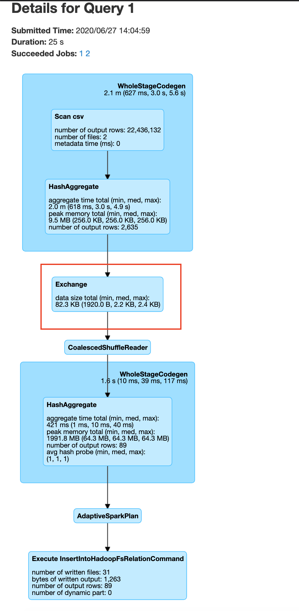
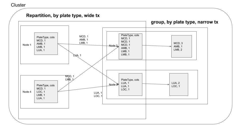
exit()

You may be wondering how we got the number 87, It is the number of unique plate type values in the plate type field. We got this from plate_type.csv file. If we do not specify 87, spark will by default set the number of partitions to 200(spark.sql.shuffle.partitions) which would negate the benefits of repartitioning. In your history server -> application UI -> SQL tab -> save query , you will be able to see the exchange happen before the groupBy as shown below

After the data exchange caused by the repartition operation we see that the data processing is done without moving data across the network, this is called a narrow transformation

Narrow Transformation

Here you repartition based on Plate Type, after which your groupby becomes a narrow transformation.

Key points

1. Data shuffle is expensive, but sometimes necessary.
2. Depending on your code logic and requirements, if you have multiple wide transformations on 1(or more) fields, you can repartition the data by that 1(or more) fields to reduce expensive data shuffles in the wide transformations.
3. Check Spark execution using .explain before actually executing the code.
4. Check the plan that was executed through History server -> spark application UI -> SQL tab -> operation.

Technique 2. Use caching, when necessary

There are scenarios where it is beneficial to cache a data frame in memory and not have to read it into memory each time. Let’s consider the previous data repartition example

pyspark --num-executors=2 # start pyspark shell

parkViolations = spark.read.option("header", True).csv("/input/")
parkViolationsPlateTypeDF = parkViolations.repartition(87, "Plate Type")
plateTypeCountDF = parkViolationsPlateTypeDF.groupBy("Plate Type").count()
plateTypeCountDF.write.format("com.databricks.spark.csv").option("header", True).mode("overwrite").save("/output/plate_type_count.csv")
# we also do a average aggregation
plateTypeAvgDF = parkViolationsPlateTypeDF.groupBy("Plate Type").avg() # avg is not meaningful here, but used just as an aggregation example
plateTypeAvgDF.write.format("com.databricks.spark.csv").option("header", True).mode("overwrite").save("/output/plate_type_avg.csv")
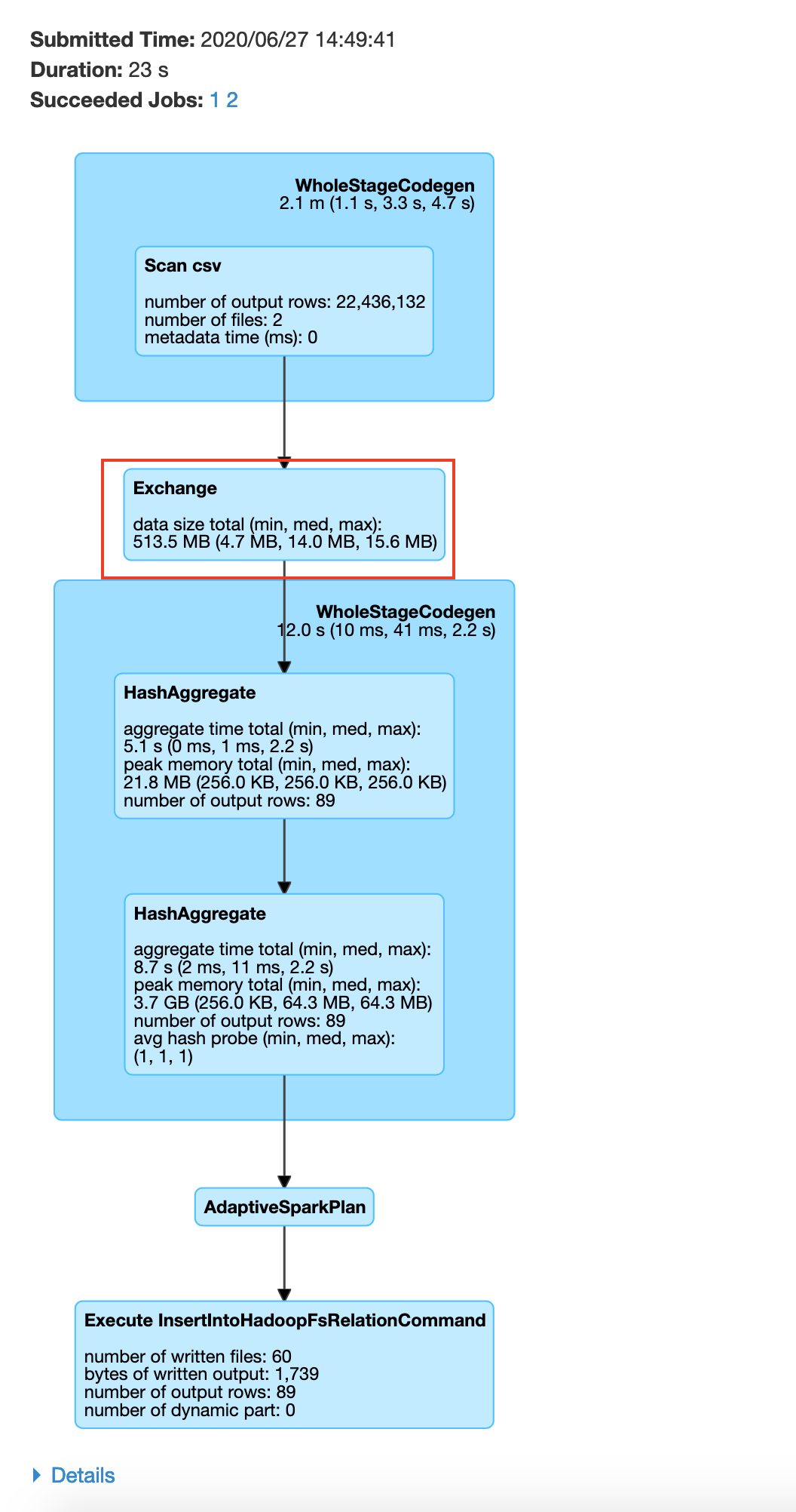
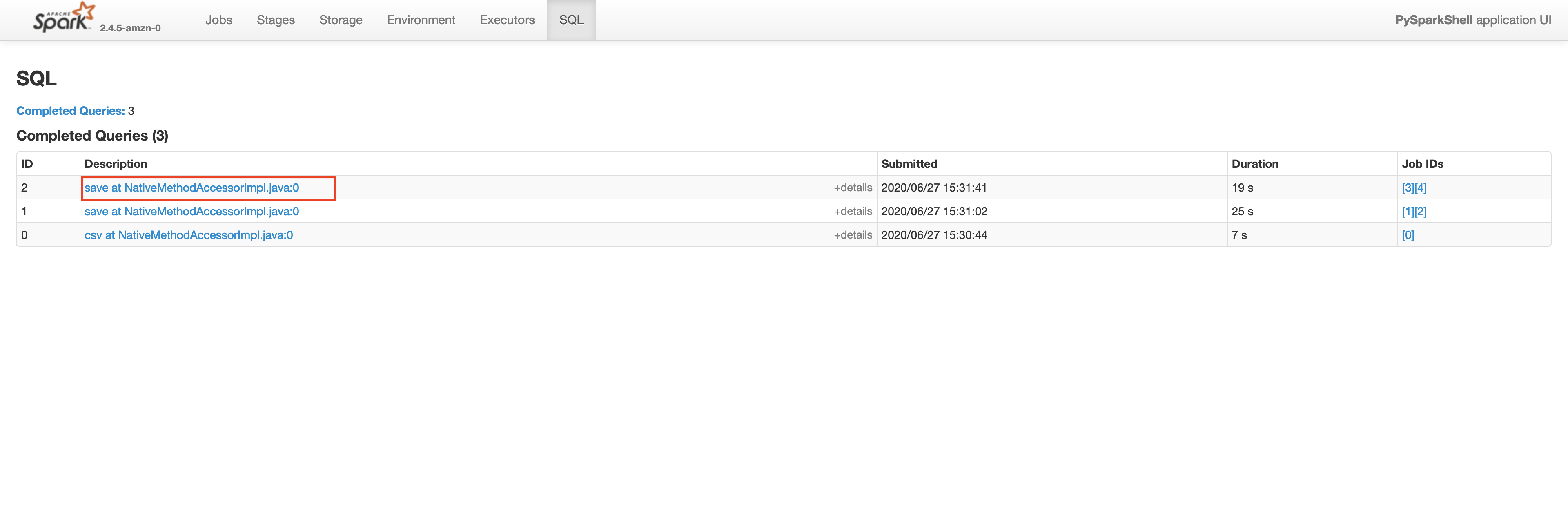
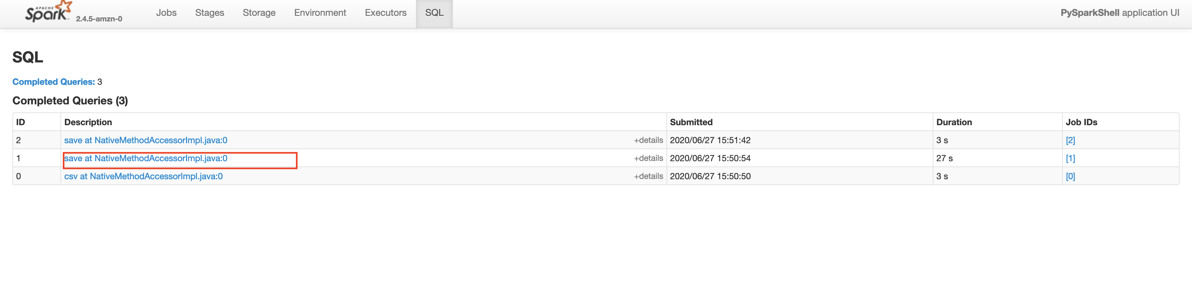
exit()

Let’s check the Spark UI for the write operation on plateTypeCountDF and plateTypeAvgDF dataframe.

Saving plateTypeCountDF without cache

Saving plateTypeAvgDF without cache

You will see that we are redoing the repartition step each time for plateTypeCountDF and plateTypeAvgDF dataframe. We can prevent the second repartition by caching the result of the first repartition, as shown below

pyspark --num-executors=2 # start pyspark shell

parkViolations = spark.read.option("header", True).csv("/input/")
parkViolationsPlateTypeDF = parkViolations.repartition(87, "Plate Type")
cachedDF = parkViolationsPlateTypeDF.select('Plate Type').cache() # we are caching only the required field of the  dataframe in memory to keep cache size small
plateTypeCountDF = cachedDF.groupBy("Plate Type").count()
plateTypeCountDF.write.format("com.databricks.spark.csv").option("header", True).mode("overwrite").save("/output/plate_type_count.csv")
# we also do a average aggregation
plateTypeAvgDF = cachedDF.groupBy("Plate Type").avg() # avg is not meaningful here, but used just as an aggregation example
plateTypeAvgDF.write.format("com.databricks.spark.csv").option("header", True).mode("overwrite").save("/output/plate_type_avg.csv")
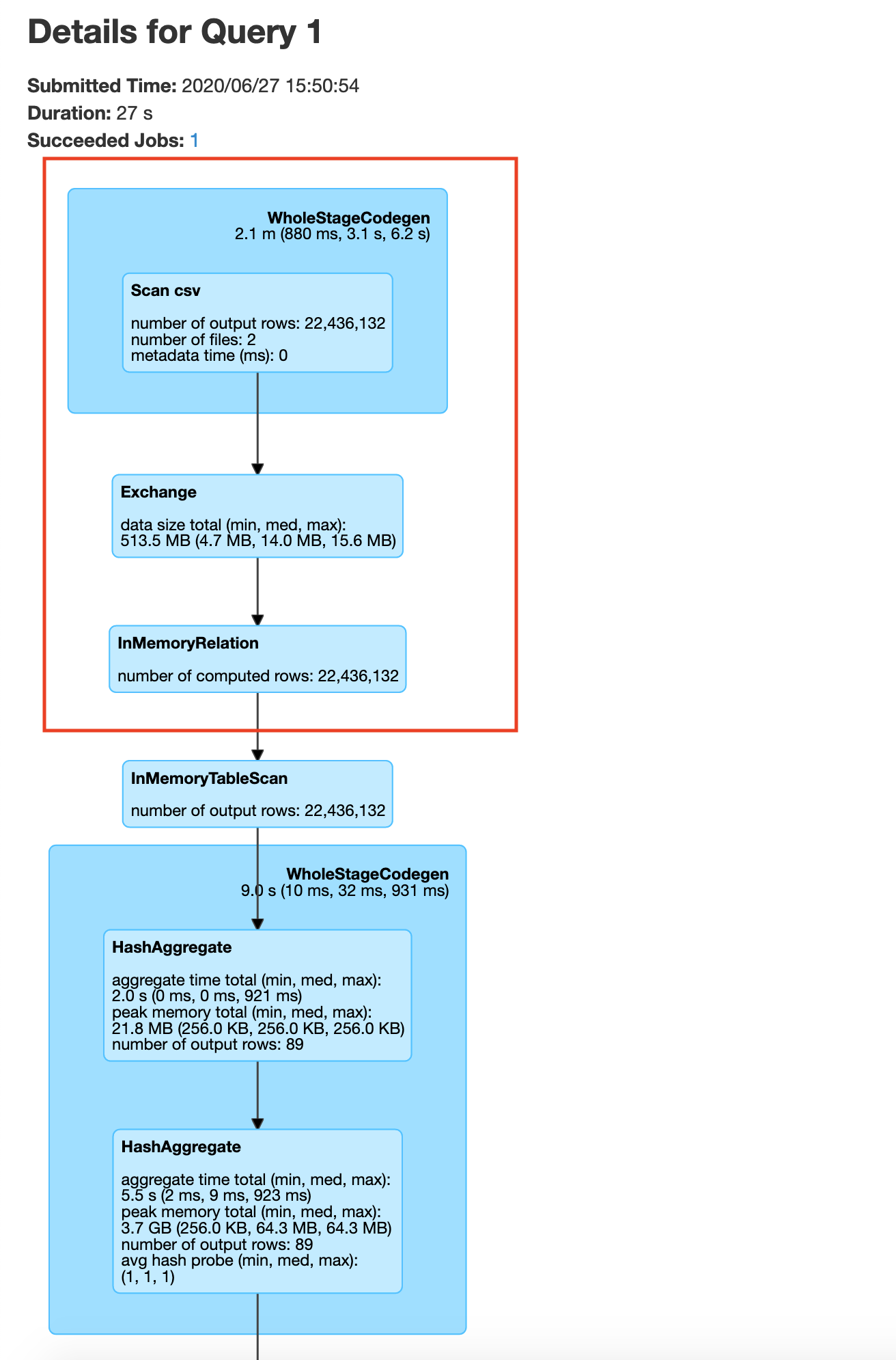
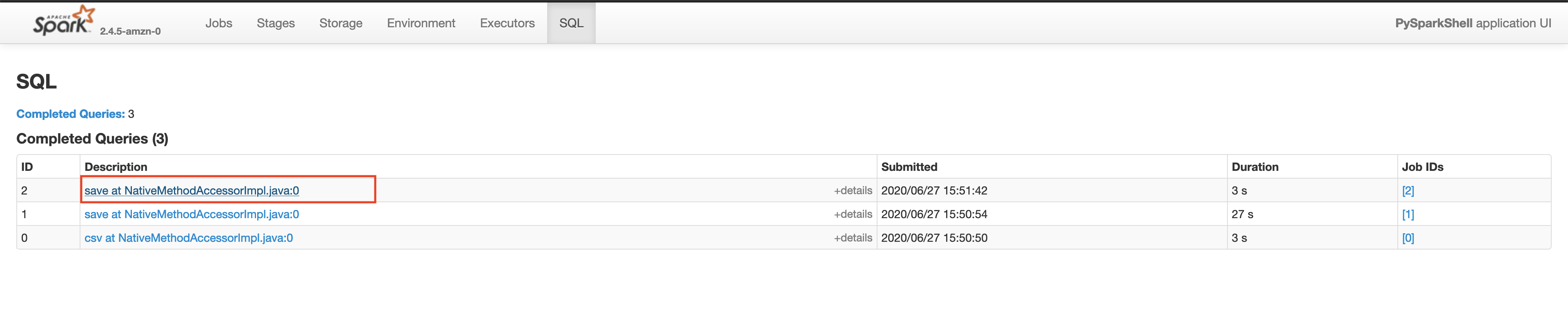
exit()

If your process involves multiple Apache Spark jobs having to read from parkViolationsPlateTypeDF you can also save it to the disk in your HDFS cluster, so that in the other jobs you can perform groupby without repartition. Let’s check the Spark UI for the write operation on plateTypeCountDF and plateTypeAvgDF dataframe.

Saving plateTypeCountDF with cache

Saving plateTypeAvgDF with cache

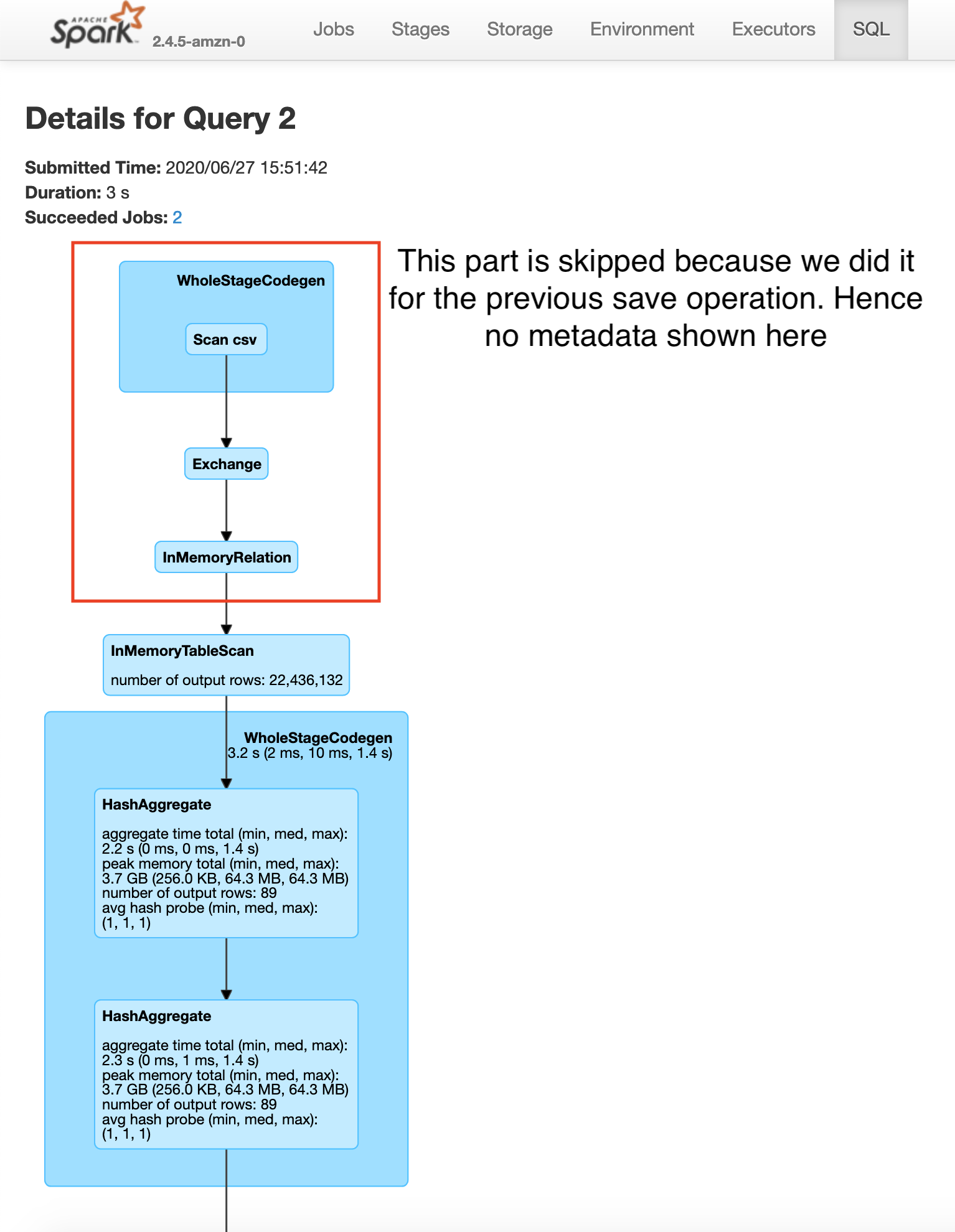
Here you will see that the construction of plateTypeAvgDF dataframe does not involve the file scan and repartition, because that dataframe parkViolationsPlateTypeDF is already in the cluster memory. Note that here we are using the clusters cache memory. For very large dataframes we can use persist method to save the dataframe using a combination of cache and disk if necessary. Caching a dataframe avoids having to re-read the dataframe into memory for processing, but the tradeoff is the fact that the Apache Spark cluster now holds an entire dataframe in memory.

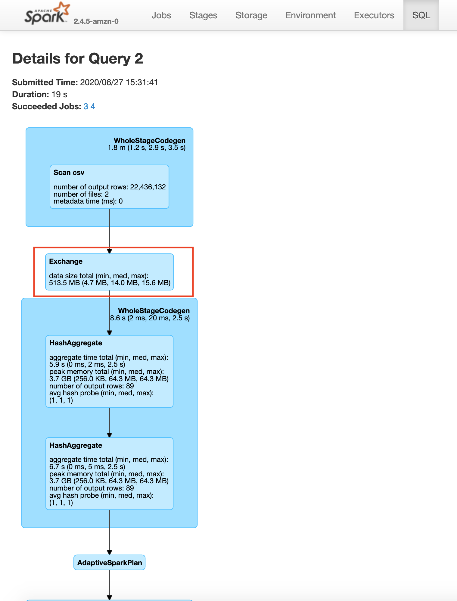
You will also see a significant increase in speed between the second save operations in the example without caching 19s vs with caching 3s.

You can visualize caching as shown below, for one node in the cluster

user exercise

Consider that you have to save the parkViolations into parkViolationsNY, parkViolationsNJ, parkViolationsCT, parkViolationsAZ depending on the Registration State field. Will caching help here, if so how?

Key points

1. If you are using a particular data frame multiple times, try caching the dataframe’s necessary columns to prevent multiple reads from disk and reduce the size of dataframe to be cached.
2. One thing to be aware of is the cache size of your cluster, do not cache data frames if not necessary.
3. The tradeoff in terms of speed is the time taken to cache your dataframe in memory.
4. If you need a way to cache a data frame part in memory and part in disk or other such variations refer to persist

Technique 3. Join strategies - broadcast join and bucketed joins

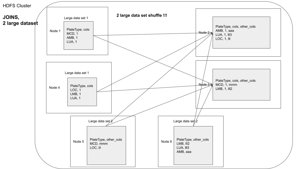
One of the most common operations in data processing is a join. When you are joining multiple datasets you end up with data shuffling because a chunk of data from the first dataset in one node may have to be joined against another data chunk from the second dataset in another node. There are 2 key techniques you can do to reduce(or even eliminate) data shuffle during joins.

3.1. Broadcast Join

Most big data joins involves joining a large fact table against a small mapping or dimension table to map ids to descriptions, etc. If the mapping table is small enough we can use broadcast join to move the mapping table to each of the node that has the fact tables data in it and preventing the data shuffle of the large dataset. This is called a broadcast join due to the fact that we are broadcasting the dimension table. By default the maximum size for a table to be considered for broadcasting is 10MB.This is set using the spark.sql.autoBroadcastJoinThreshold variable. First lets consider a join without broadcast.

hdfs dfs -rm -r /output # free up some space in HDFS
pyspark --num-executors=2 # start pyspark shell

parkViolations_2015 = spark.read.option("header", True).csv("/input/2015.csv")
parkViolations_2016 = spark.read.option("header", True).csv("/input/2016.csv")

parkViolations_2015 = parkViolations_2015.withColumnRenamed("Plate Type", "plateType") # simple column rename for easier joins
parkViolations_2016 = parkViolations_2016.withColumnRenamed("Plate Type", "plateType")

parkViolations_2016_COM = parkViolations_2016.filter(parkViolations_2016.plateType == "COM")
parkViolations_2015_COM = parkViolations_2015.filter(parkViolations_2015.plateType == "COM")

joinDF = parkViolations_2015_COM.join(parkViolations_2016_COM, parkViolations_2015_COM.plateType ==  parkViolations_2016_COM.plateType, "inner").select(parkViolations_2015_COM["Summons Number"], parkViolations_2016_COM["Issue Date"])
joinDF.explain() # you will see SortMergeJoin, with exchange for both dataframes, which means involves data shuffle of both dataframe
# The below join will take a very long time with the given infrastructure, do not run, unless needed
# joinDF.write.format("com.databricks.spark.csv").option("header", True).mode("overwrite").save("/output/joined_df")
exit()

The above process will be very slow, since it involves distributing 2 large datasets and then joining

In order to prevent the data shuffle of 2 large datasets, you can optimize your code to enable broadcast join, as shown below

hdfs dfs -rm -r /output # free up some space in HDFS
pyspark --num-executors=2 # start pyspark shell

parkViolations_2015 = spark.read.option("header", True).csv("/input/2015.csv")
parkViolations_2016 = spark.read.option("header", True).csv("/input/2016.csv")

parkViolations_2015 = parkViolations_2015.withColumnRenamed("Plate Type", "plateType") # simple column rename for easier joins
parkViolations_2016 = parkViolations_2016.withColumnRenamed("Plate Type", "plateType")

parkViolations_2015_COM = parkViolations_2015.filter(parkViolations_2015.plateType == "COM").select("plateType", "Summons Number").distinct()
parkViolations_2016_COM = parkViolations_2016.filter(parkViolations_2016.plateType == "COM").select("plateType", "Issue Date").distinct()

parkViolations_2015_COM.cache()
parkViolations_2016_COM.cache()

parkViolations_2015_COM.count() # will cause parkViolations_2015_COM to be cached
parkViolations_2016_COM.count() # will cause parkViolations_2016_COM to be cached

joinDF = parkViolations_2015_COM.join(parkViolations_2016_COM.hint("broadcast"), parkViolations_2015_COM.plateType ==  parkViolations_2016_COM.plateType, "inner").select(parkViolations_2015_COM["Summons Number"], parkViolations_2016_COM["Issue Date"])
joinDF.explain() # you will see BroadcastHashJoin

joinDF.write.format("com.databricks.spark.csv").option("header", True).mode("overwrite").save("/output/joined_df")
exit()

In the Spark SQL UI you will see the execution to follow a broadcast join.

In some cases if one of the dataframe is small Spark automatically switches to use broadcast join as shown below.

parkViolations = spark.read.option("header", True).csv("/input/")
plateType = spark.read.schema("plate_type_id STRING, plate_type STRING").csv("/mapping/plate_type.csv")
parkViolations = parkViolations.withColumnRenamed("Plate Type", "plateType") # simple column rename for easier joins
joinDF = parkViolations.join(plateType, parkViolations.plateType ==  plateType.plate_type_id, "inner")
joinDF.write.format("com.databricks.spark.csv").option("header", True).mode("overwrite").save("/output/joined_df.csv")
exit()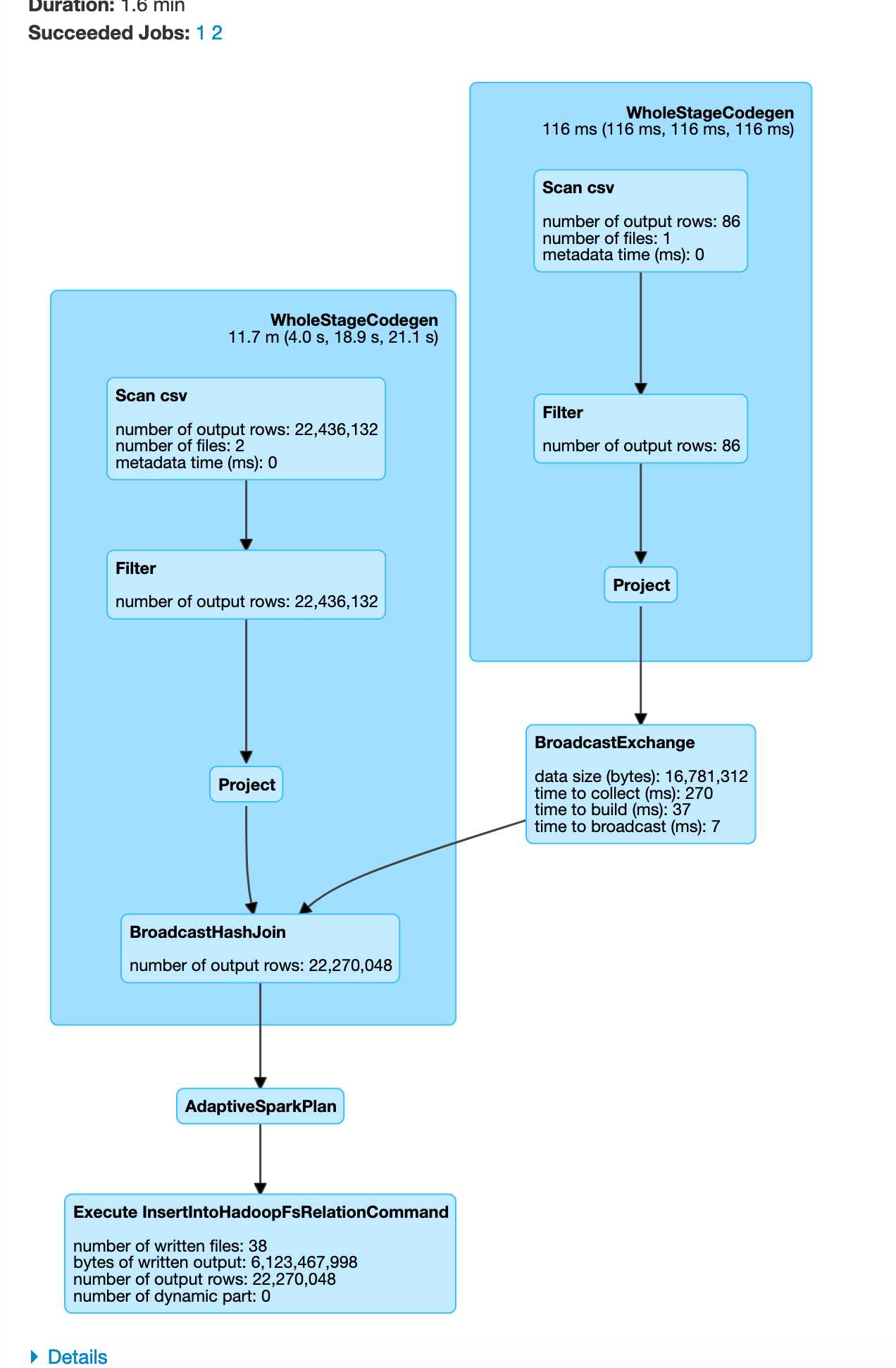

You can visualize this as

In this example since our plateType dataframe is already small, Apache Spark auto optimizes and chooses to use a broadcast join. From the above you can see how we can do a broadcast join to reduce the data moved over the network.

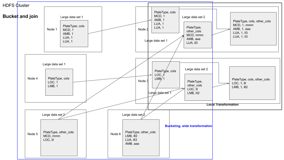
3.2. Bucketed Join

In an example above we joined parkViolations_2015 and parkViolations_2016, but only kept certain columns and only after removing duplicates. What if we need to do joins in the future based on the plateType field but we might need most (if not all) of the columns, as required by our program logic.

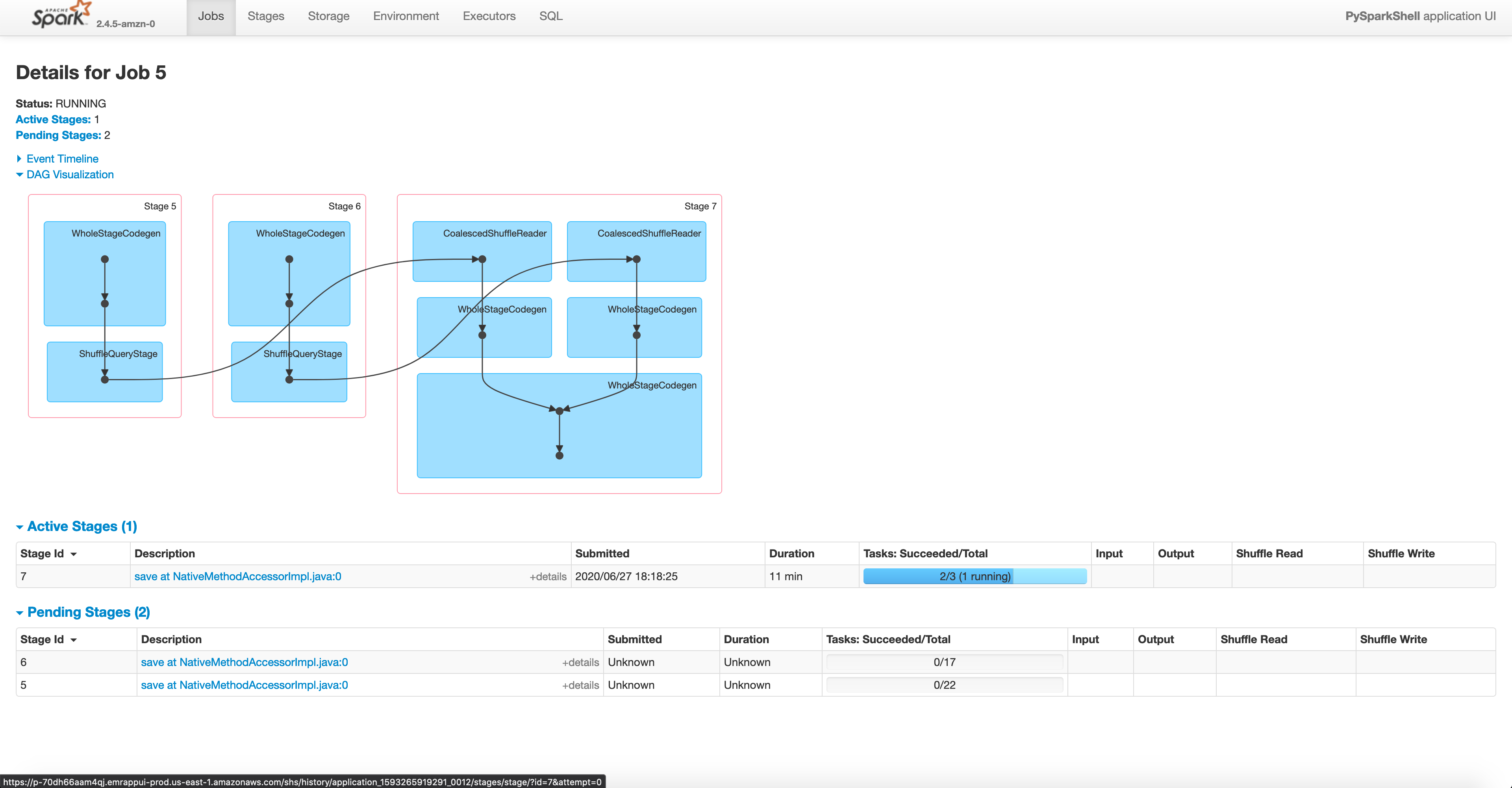
You can visualize it as shown below

A basic approach would be to repartition one dataframe by the field on which the join is to be performed and then join with the second dataframe, this would involve data shuffle for the second dataframe at transformation time.

Another approach would be to use bucketed joins. Bucketing is a technique which you can use to repartition a dataframe based on a field. If you bucket both the dataframe based on the filed that they are supposed to be joined on, it will result in both the dataframes having their data chunks to be made available in the same nodes for joins, because the location of nodes are chosen using the hash of the partition field.

You can visualize bucketed join as shown below

hdfs dfs -rm -r /output # free up some space in HDFS
pyspark --num-executors=2 --executor-memory=8g # start pyspark shell

parkViolations_2015 = spark.read.option("header", True).csv("/input/2015.csv")
parkViolations_2016 = spark.read.option("header", True).csv("/input/2016.csv")

new_column_name_list= list(map(lambda x: x.replace(" ", "_"), parkViolations_2015.columns))

parkViolations_2015 = parkViolations_2015.toDF(*new_column_name_list)
parkViolations_2015 = parkViolations_2015.filter(parkViolations_2015.Plate_Type == "COM").filter(parkViolations_2015.Vehicle_Year == "2001")
parkViolations_2016 = parkViolations_2016.toDF(*new_column_name_list)
parkViolations_2016 = parkViolations_2016.filter(parkViolations_2016.Plate_Type == "COM").filter(parkViolations_2016.Vehicle_Year == "2001")
# we filter for COM and 2001 to limit time taken for the join

spark.conf.set("spark.sql.autoBroadcastJoinThreshold", -1) # we do this so that Spark does not auto optimize for broadcast join, setting to -1 means disable

parkViolations_2015.write.mode("overwrite").bucketBy(400, "Vehicle_Year", "plate_type").saveAsTable("parkViolations_bkt_2015")
parkViolations_2016.write.mode("overwrite").bucketBy(400, "Vehicle_Year", "plate_type").saveAsTable("parkViolations_bkt_2016")

parkViolations_2015_tbl = spark.read.table("parkViolations_bkt_2015")
parkViolations_2016_tbl = spark.read.table("parkViolations_bkt_2016")

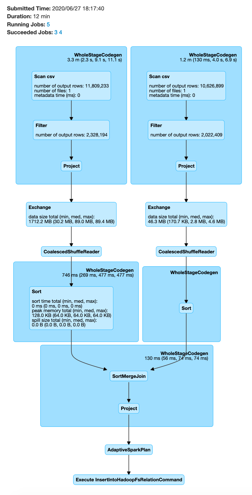
joinDF = parkViolations_2015_tbl.join(parkViolations_2016_tbl, (parkViolations_2015_tbl.Plate_Type ==  parkViolations_2016_tbl.Plate_Type) & (parkViolations_2015_tbl.Vehicle_Year ==  parkViolations_2016_tbl.Vehicle_Year) , "inner").select(parkViolations_2015_tbl["Summons_Number"], parkViolations_2016_tbl["Issue_Date"])

joinDF.explain() # you will see SortMergeJoin, but no exchange, which means no data shuffle

# The below join will take a while, approx 30min
joinDF.write.format("com.databricks.spark.csv").option("header", True).mode("overwrite").save("/output/bkt_joined_df.csv")
exit()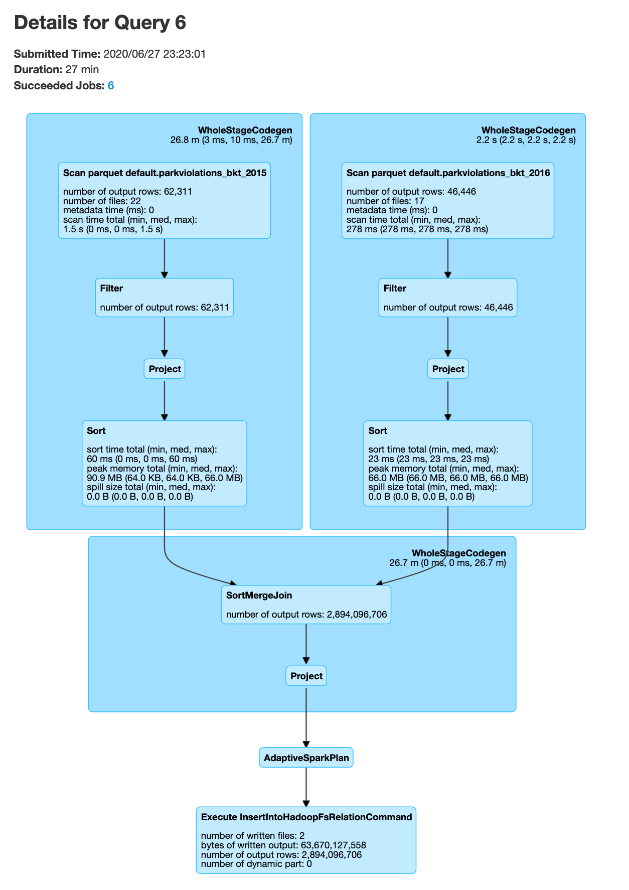

Note that in the above code snippet we start pyspark with --executor-memory=8g this option is to ensure that the memory size for each node is 8GB due to the fact that this is a large join. The number of buckets 400 was chosen to be an arbritray large number.

The write.bucketBy writes to our HDFS at /user/spark/warehouse/. You can check this using

hdfs dfs -ls /user/spark/warehouse/

user exercise

Try bucketed join but with different bucket sizes > 400 and < 400. How does it affect performance? Why? Can you use repartition to achieve same or similar result? If you execute the write in the bucketed tables example you will notice there will b e one executor at the end that takes up most of the time, why is this? how can it be prevented?

Key points

1. If one of your table is much smaller compared to the other, consider using broadcast join
2. If you want to avoid data shuffle during the join query time, but are ok with pre shuffling the data, consider using the bucketed join technique.
3. Bucketing increases performance with discrete columns(ie columns with limited number of unique values, in our case the plate type column has 87 distinct values), if the values are continuous(or have high number of unique values) the performance boost may not be worth it.

TL; DR

1. Reduce data shuffle, use repartition to organize dataframes to prevent multiple data shuffles.
2. Use caching, when necessary to keep data in memory to save on disk read costs.
3. Optimize joins to prevent data shuffles, using broadcast technique or bucket join techniques.
4. There is no one size fits all solution for optimizing Spark, use the above techniques to choose the optimal strategy for your use case.

Conclusion

These are some techniques that help you resolve most(usually 80%) of your Apache Spark performance issues. Knowing when to use them and when not to use them is crucial, eg. you might not want to use caching if that data frame is used for only one transformation. There are more techniques like key salting for dealing with data skew, etc. But the fundamental concept is to make a tradeoff between preprocessing the data to prevent data shuffles and then performing transformations as necessary depending on your use case.

Hope this post provides you some ways to think about optimizing your spark code. Please let me know if you have any questions or comments in the comment section below.

Reference:

1. Spark Docs
2. Bucketing
3. Data