1. Introduction
An actual data engineering project usually involves multiple components. Setting up a data engineering project while conforming to best practices can be highly time-consuming. If you are
A data analyst, student, scientist, or engineer looking to gain data engineering experience but cannot find a good starter project.
Wanting to work on a data engineering project that simulates a real-life project.
Looking for an end-to-end data engineering project.
Looking for a good project to get data engineering experience for job interviews.
Then this tutorial is for you. In this tutorial, you will
Set up Apache Airflow, Apache Spark, DuckDB, and Minio (OSS S3).
Learn data pipeline best practices.
Learn how to spot failure points in data pipelines and build systems resistant to failures.
Learn how to design and build a data pipeline from business requirements.
If you are interested in a stream processing project, please check out Data Engineering Project for Beginners - Stream Edition.
2. Objective
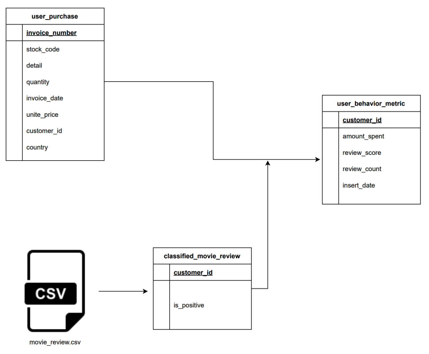
Suppose you work for a user behavior analytics company that collects user data and creates a user profile. We are tasked with building a data pipeline to populate the user_behavior_metric table. The user_behavior_metric table is an OLAP table used by analysts, dashboard software, etc. It is built from
user_purchase: OLTP table with user purchase information.movie_review.csv: Data is sent every day by an external data vendor.
3. Run Data Pipeline
Code available at beginner_de_project repository.
3.1. Run on codespaces
You can run this data pipeline using GitHub codespaces. Follow the instructions below.
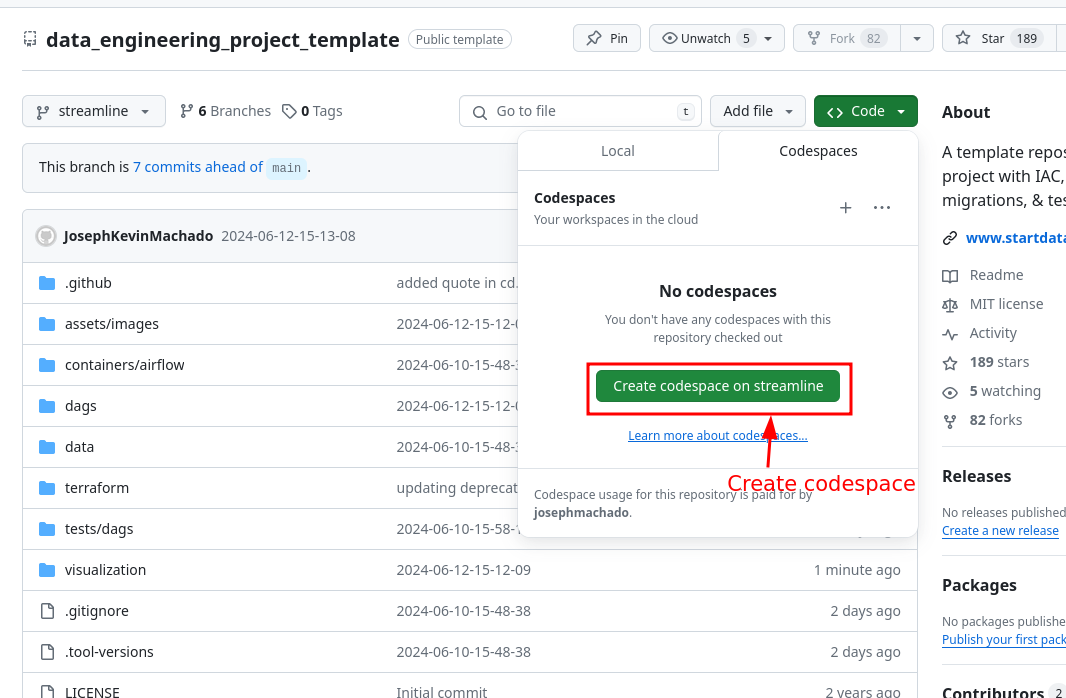
- Create codespaces by going to the beginner_de_project repository, cloning it(or clicking the
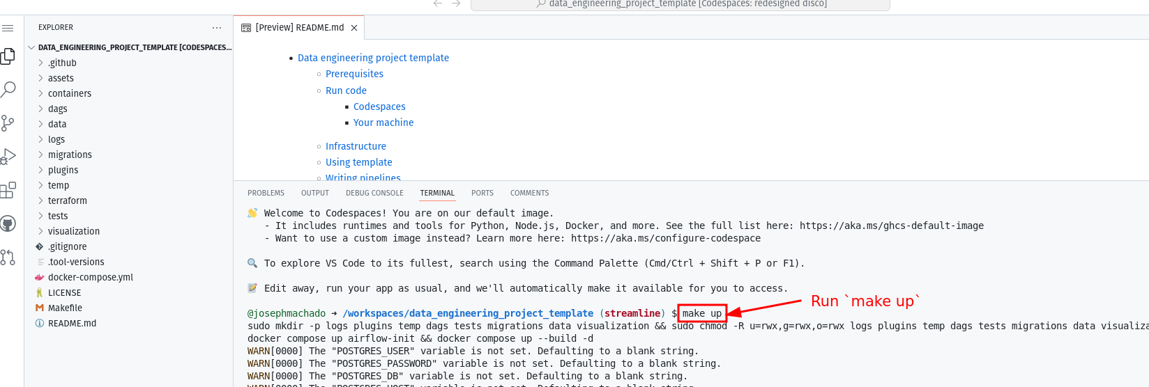
Use this templatebutton), and then clicking theCreate codespaces on mainbutton. - Wait for codespaces to start, then in the terminal type
make up. - Wait for
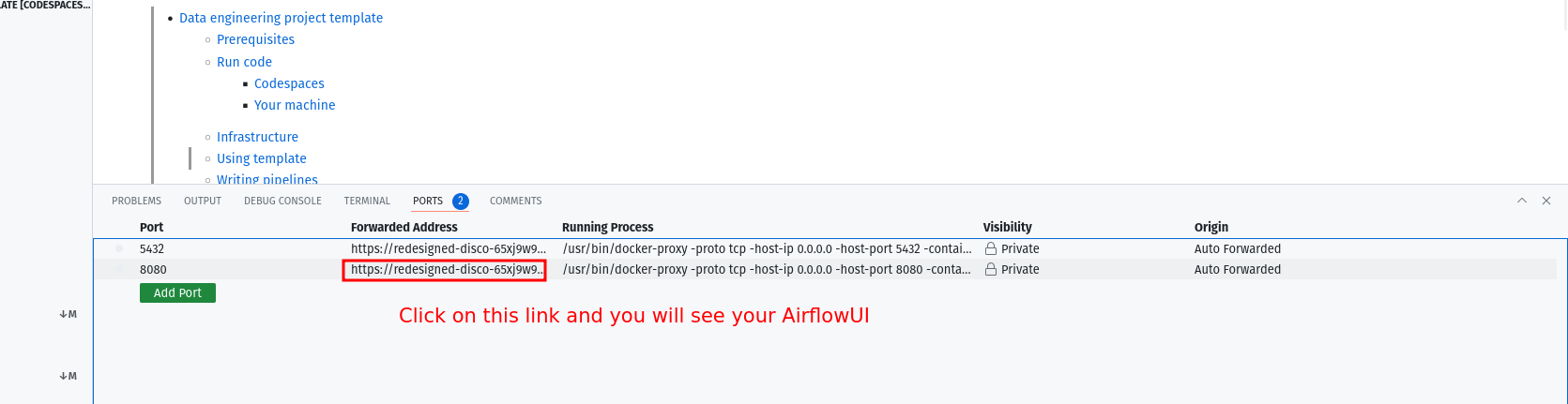
make upto complete, and then wait for 30s (for Airflow to start). - After 30 seconds, go to the
portstab and click on the link exposing port8080to access the Airflow UI (your username and password areairflow).
3.2. Run locally
To run locally, you need:
- git
- Github account
- Docker with at least 4GB of RAM and Docker Compose v1.27.0 or later
Clone the repo and run the following commands to start the data pipeline:
Go to http:localhost:8080 to see the Airflow UI. The username and password are both airflow.
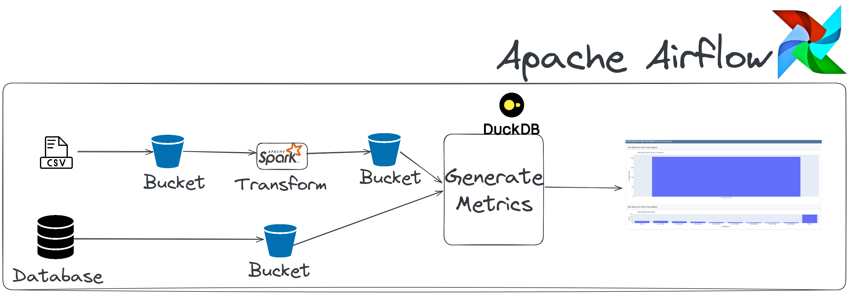
4. Architecture
This data engineering project includes the following:
Airflow: To schedule and orchestrate DAGs.Postgres: This database stores Airflow’s details (which you can see via the Airflow UI) and has a schema to represent upstream databases.DuckDB: To act as our warehouseQuarto with Plotly: To convert code inmarkdownformat to HTML files that can be embedded in your app or served as is.Apache Spark: This is used to process our data, specifically to run a classification algorithm.minio: To provide an S3 compatible open source storage system.
For simplicity, services 1-5 of the above are installed and run in one container defined here.
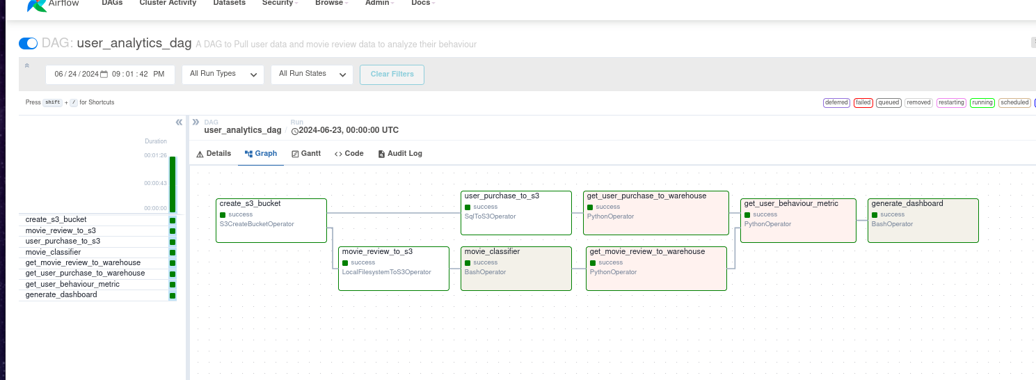
The user_analytics_dag DAG in the Airflow UI will look like the below image:
On completion, you can see the dashboard html rendered at dags/scripts/dashboard/dashboard.html.
Read this postfor information on setting up CI/CD, IAC(terraform), “make” commands, and automated testing.
5. Code walkthrough
The data for user_behavior_metric is generated from 2 primary datasets. We will examine how each is ingested, transformed, and used to get the data for the final table.
5.1 Extract user data and movie reviews
We extract data from two sources.
User purchase informationfrom a csv file. We useLocalFileSystemToS3Operatorfor this extraction.Movie reviewdata containing information about how a user reviewed a movie from a Postgres database. We useSqlToS3Operatorfor this extraction.
We use Airflow’s native operators to extract data as shown below (code link):
movie_review_to_s3 = LocalFilesystemToS3Operator(
    task_id="movie_review_to_s3",
    filename="/opt/airflow/data/movie_review.csv",
    dest_key="raw/movie_review.csv",
    dest_bucket=user_analytics_bucket,
    replace=True,
)

user_purchase_to_s3 = SqlToS3Operator(
    task_id="user_purchase_to_s3",
    sql_conn_id="postgres_default",
    query="select * from retail.user_purchase",
    s3_bucket=user_analytics_bucket,
    s3_key="raw/user_purchase/user_purchase.csv",
    replace=True,
)
5.2. Classify movie reviews and create user metrics
We use Spark to classify reviews as positive or negative, and ML and DuckDB are used to generate metrics with SQL.
The code is shown below (code link):
    movie_classifier = BashOperator(
        task_id="movie_classifier",
        bash_command="python /opt/airflow/dags/scripts/spark/random_text_classification.py",
    )

    get_movie_review_to_warehouse = PythonOperator(
        task_id="get_movie_review_to_warehouse",
        python_callable=get_s3_folder,
        op_kwargs={"s3_bucket": "user-analytics", "s3_folder": "clean/movie_review"},
    )

    get_user_purchase_to_warehouse = PythonOperator(
        task_id="get_user_purchase_to_warehouse",
        python_callable=get_s3_folder,
        op_kwargs={"s3_bucket": "user-analytics", "s3_folder": "raw/user_purchase"},
    )

    def create_user_behaviour_metric():
        q = """
        with up as (
          select
            *
          from
            '/opt/airflow/temp/s3folder/raw/user_purchase/user_purchase.csv'
        ),
        mr as (
          select
            *
          from
            '/opt/airflow/temp/s3folder/clean/movie_review/*.parquet'
        )
        select
          up.customer_id,
          sum(up.quantity * up.unit_price) as amount_spent,
          sum(
            case when mr.positive_review then 1 else 0 end
          ) as num_positive_reviews,
          count(mr.cid) as num_reviews
        from
          up
          join mr on up.customer_id = mr.cid
        group by
          up.customer_id
        """
        duckdb.sql(q).write_csv("/opt/airflow/data/behaviour_metrics.csv")
We use a naive Spark ML implementation(random_text_classification) to classify reviews.
5.3. Load data into the destination
We store the calculated user behavior metrics at /opt/airflow/data/behaviour_metrics.csv. The data stored as csv is used by downstream consumers, such as our dashboard generator.
5.4. See how the data is distributed
We create visualizations using a tool called quarto, which enables us to write Python code to generate HTML files that display the charts.
We use Airflow’s BashOperator to create our dashboard, as shown below:
You can modify the code to generate dashboards.
6. Design considerations
Read the following articles before answering these design considerations.
Now that you have the data pipeline running successfully, it’s time to review some design choices.
Idempotent data pipeline
Check that all the tasks are idempotent. If you re-run a partially run or a failed task, your output should not be any different than if the task had run successfully. Read this article to understand idempotency in detail.
Hint, there is at least one non-idempotent task.Monitoring & Alerting
The data pipeline can be monitored from the Airflow UI. Spark can be monitored via the Spark UI. We do not have any alerts for task failures, data quality issues, hanging tasks, etc. In real projects, there is usually a monitoring and alerting system. Some common systems used for monitoring and alerting are
cloud watch,datadog, ornewrelic.Quality control
We do not check for data quality in this data pipeline. We can set up basic count, standard deviation, etc, checks before we load data into the final table for advanced testing requirements consider using a data quality framework, such as great_expectations. For a lightweight solution take a look at this template that uses the cuallee library for data quality checks.
Concurrent runs
If you have to re-run the pipeline for the past three months, it would be ideal to have them run concurrently and not sequentially. We can set levels of concurrency as shown here. Even with an appropriate concurrency setting, our data pipeline has one task that is blocking. Figuring out the blocking task is left as an exercise for the reader.
Changing DAG frequency
What changes are necessary to run this DAG every hour? How will the table schema need to change to support this? Do you have to rename the DAG?
Backfills
Assume you have a logic change in the movie classification script. You want this change to be applied to the past three weeks. If you want to re-run the data pipeline for the past three weeks, will you
re-run the entire DAG or only parts of it. Why would you choose one option over the other? You can use this command to run backfills.Data size
Will the data pipeline run successfully if your data size increases by 10x, 100x, or 1000x why? Why not? Please read - how to scale data pipelines on how to do this.
7. Next steps
If you want to work more with this data pipeline, please consider contributing to the following.
- Unit tests, DAG run tests, and integration tests.
- Add CI/CD steps following the data engineering template
If you have other ideas, please feel free to open Github issues or pull requests.
8. Conclusion
This article gives you a good idea of how to design and build an end-to-end data pipeline. To recap, we saw:
- Infrastructure setup
- Data pipeline best practices
- Design considerations
- Next steps
Please leave any questions or comments in the comment section below.