What are Common Table Expressions(CTEs) and when to use them?

Oct 12, 2021 · 8 min read

Introduction
Setup
Common Table Expressions (CTEs)
Performance comparison
Tear down
Conclusion
References

Introduction

If you are a student, analyst, engineer, or anyone in the data space and are

Wondering what CTEs are?

Trying to understand CTE performance

Then this post is for you. In this post, we go over what CTEs are and compare their performance to the subquery, derived table, and temp table.

Setup

This post uses AWS Redshift to explore CTEs. You can follow along without having to set up your Redshift instance as well.

Prerequisites

Let’s create a Redshift instance using the AWS cli.

# create an AWS Redshift instance
aws redshift create-cluster --node-type dc2.large --number-of-nodes 2 --master-username sdeuser --master-user-password Password1234 --cluster-identifier sdeSampleCluster

# get your AWS Redshift endpoints address
aws redshift describe-clusters --cluster-identifier sdesamplecluster | grep '\"Address'

# use pgcli to connect to your AWS Redshift instance
pgcli -h <your-redshift-address> -U sdeuser -p 5439 -d dev
# note dev is the default database created. When prompted for the password enter "Password1234".

Let’s assume you work for a data collection company that tracks user clickstream and geolocation data. In your SQL terminal, create fake clickstream and geolocation tables as shown below.

-- create fake clickstream data
drop table if exists clickstream;
create table clickstream (
    eventId varchar(40),
    userId int,
    sessionId int,
    actionType varchar(8),
    datetimeCreated timestamp
);
insert into clickstream(eventId, userId, sessionId, actionType, datetimeCreated )
values 
('6e598ae5-3fb1-476d-9787-175c34dcfeff',1 ,1000,'click','2020-11-25 12:40:00'),
('0c66cf8c-0c00-495b-9386-28bc103364da',1 ,1000,'login','2020-11-25 12:00:00'),
('58c021ad-fcc8-4284-a079-8df0d51601a5',1 ,1000,'click','2020-11-25 12:10:00'),
('85eef2be-1701-4f7c-a4f0-7fa7808eaad1',1 ,1001,'buy',  '2020-11-22 18:00:00'),
('08dd0940-177c-450a-8b3b-58d645b8993c',3 ,1010,'buy',  '2020-11-20 01:00:00'),
('db839363-960d-4319-860d-2c9b34558994',10,1120,'click','2020-11-01 13:10:03'),
('2c85e01d-1ed4-4ec6-a372-8ad85170a3c1',10,1121,'login','2020-11-03 18:00:00'),
('51eec51c-7d97-47fa-8cb3-057af05d69ac',8 ,6,   'click','2020-11-10 10:45:53'),
('5bbcbc71-da7a-4d75-98a9-2e9bfdb6f925',3 ,3002,'login','2020-11-14 10:00:00'),
('f3ee0c19-a8f9-4153-b34e-b631ba383fad',1 ,90,  'buy',  '2020-11-17 07:00:00'),
('f458653c-0dca-4a59-b423-dc2af92548b0',2 ,2000,'buy',  '2020-11-20 01:00:00'),
('fd03f14d-d580-4fad-a6f1-447b8f19b689',2 ,2000,'click','2020-11-20 00:00:00');

-- create fake geolocation data
drop table if exists geolocation;
create table geolocation (
    userId int,
    zipcode varchar(10),
    datetimeCreated timestamp
);

insert into geolocation(userId, zipCode, datetimeCreated )
values 
(1 ,66206,'2020-11-25 12:40:00'),
(1 ,66209,'2020-11-25 12:00:00'),
(1 ,91355,'2020-11-25 12:10:00'),
(1 ,83646,'2020-11-22 18:00:00'),
(3 ,91354,'2020-11-20 01:00:00'),
(10,91355,'2020-11-01 13:10:03'),
(10,91355,'2020-11-03 18:00:00'),
(8 ,91355,'2020-11-10 10:45:53'),
(3 ,91355,'2020-11-14 10:00:00'),
(1 ,83646,'2020-11-17 07:00:00'),
(2 ,83646,'2020-11-20 01:00:00'),
(2 ,91355,'2020-11-20 00:00:00');

Common Table Expressions (CTEs)

Let’s assume we want to calculate the number of purchases made by active users. Active users are defined as users who have been in multiple locations (identified by zip code) and have purchased at least one product.

You can write a query that uses a subquery (where userId in (...)) as shown below.

select userId,
    sum(
        case
            when actionType = 'buy' then 1
            else 0
        end
    ) as numPurchases
from clickstream
where userId in (
        select userId
        from geolocation
        group by userId
        having count(distinct zipCode) > 1
    )
group by userId
having numPurchases >= 1;

Alternatively, we can use CTEs to define temp tables that only exist for the duration of the query as shown below.

with buyingUsers as (
    select userId,
        sum(
            case
                when actionType = 'buy' then 1
                else 0
            end
        ) as numPurchases
    from clickstream
    group by userId
    having numPurchases >= 1
),
movingUsers as (
    select userId
    from geolocation
    group by userId
    having count(distinct zipCode) > 1
)
select bu.userId,
    bu.numPurchases
from buyingUsers bu
    join movingUsers mu on bu.userId = mu.userId;

We replaced the subquery and conditional sum logic with CTE. This example is simple but in cases with multiple derived tables and sophisticated join logic, using CTEs may make your query easier to read.

Performance comparison

Now that we know what CTEs are, let’s compare their performance with approaches. Let’s use ANALYZE to update the table statistics. This will ensure that the query planner comes up with the most efficient plan to process data.

analyze clickstream;
analyze geolocation;

Let’s assume we want to calculate the number of clicks, logins, and purchases per user session for active users. Active users are defined as users who have been in multiple locations (identified by zip code) and have purchased at least one product.

The result should be

userId	sessionId	numclicks	numlogins	numpurchases
2	2000	1	0	1
1	90	0	0	1
1	1001	0	0	1
1	1000	2	1	0
3	3002	0	1	0
3	1010	0	0	1

CTE

CTE-based approach to calculate the number of clicks, logins, and purchases per user session for active users is shown below.

with purchasingUsers as (
    select userId,
        sum(
            case
                when actionType = 'buy' then 1
                else 0
            end
        ) as numPurchases
    from clickstream
    group by userId
    having numPurchases >= 1
),
movingUsers as (
    select userId
    from geolocation
    group by userId
    having count(distinct zipCode) > 1
),
userSessionMetrics as (
    select userId,
        sessionId,
        sum(
            case
                when actionType = 'click' then 1
                else 0
            end
        ) as numclicks,
        sum(
            case
                when actionType = 'login' then 1
                else 0
            end
        ) as numlogins,
        sum(
            case
                when actionType = 'buy' then 1
                else 0
            end
        ) as numPurchases
    from clickstream
    group by userId,
        sessionId
)
select usm.*
from userSessionMetrics as usm
    join movingUsers as mu on usm.userId = mu.userId
    join purchasingUsers as pu on usm.userId = pu.userId;

We can see the query plan by running explain + the above query in your sql terminal.

CTE query plan

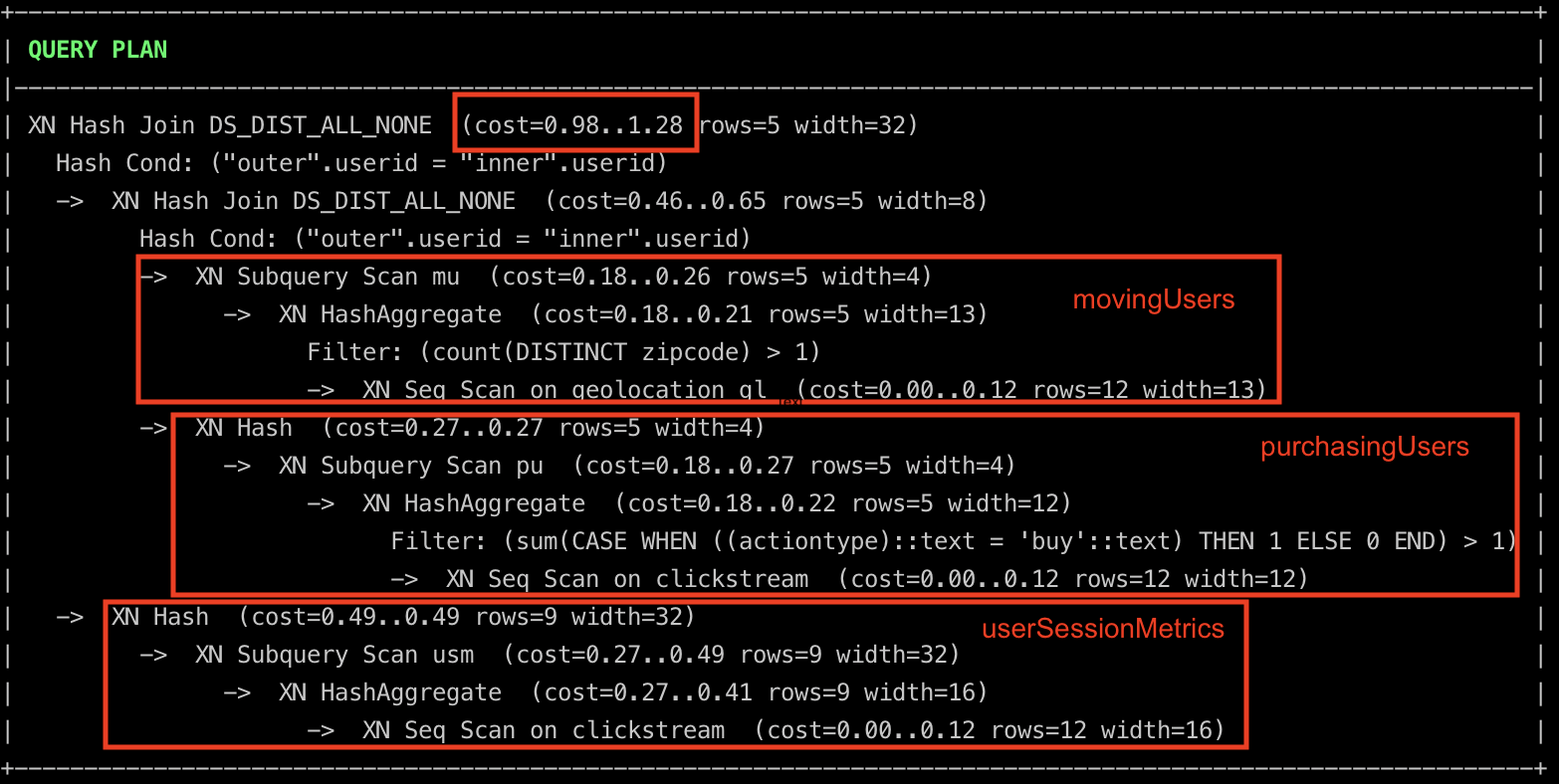
From the query plan, we can see that the query planner decided to

Calculate movingUsers and purchasingUsers in parallel and join them.
While simultaneously aggregating clickstream data to generate userSessionMetrics.
Finally, join the datasets from the above 2 points.

See cost definition here.

Subquery and derived tables

Calculating the number of clicks, logins, and purchases per user session for active users using subquery and derived tables is shown below.

select userSessionMetrics.userId,
    userSessionMetrics.sessionId,
    userSessionMetrics.numclicks,
    userSessionMetrics.numlogins,
    userSessionMetrics.numPurchases
from (
        select userId,
            sum(
                case
                    when actionType = 'buy' then 1
                    else 0
                end
            ) as numPurchases
        from clickstream
        group by userId
        having numPurchases >= 1
    ) purchasingUsers
    join (
        select userId,
            sessionId,
            sum(
                case
                    when actionType = 'click' then 1
                    else 0
                end
            ) as numclicks,
            sum(
                case
                    when actionType = 'login' then 1
                    else 0
                end
            ) as numlogins,
            sum(
                case
                    when actionType = 'buy' then 1
                    else 0
                end
            ) as numPurchases
        from clickstream
        group by userId,
            sessionId
    ) userSessionMetrics on purchasingUsers.userId = userSessionMetrics.userId
where purchasingUsers.userId in (
        select userId
        from geolocation
        group by userId
        having count(distinct zipCode) > 1
    );

We can see the query plan by running explain + the above query in your sql terminal.

sq dt query plan

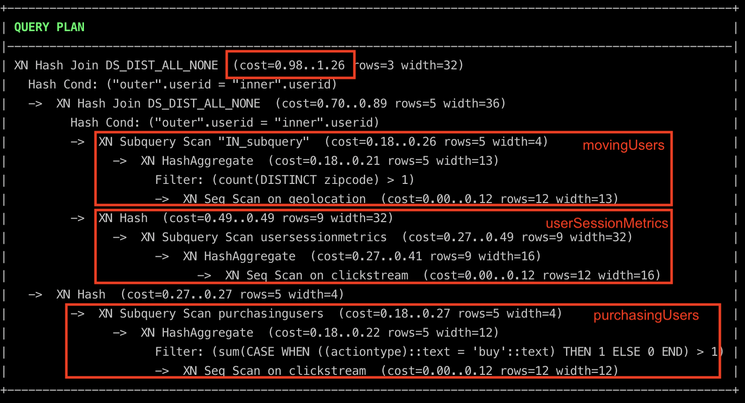
From the query plan, we can see that the query planner decided to

Calculate movingUsers (the IN subquery) and userSessionMetrics in parallel and join them.
While simultaneously filtering clickstream data to generate purchasingUsers.
Finally, join the datasets from the above 2 points.

You can see that the query plan is very similar to the CTE approach.

Temp table

Temp table-based approach to calculate the number of clicks, logins, and purchases per user session for active users is shown below.

create temporary table purchasingUsers DISTKEY(userId) as (
    select userId,
        sum(
            case
                when actionType = 'buy' then 1
                else 0
            end
        ) as numPurchases
    from clickstream
    group by userId
    having numPurchases >= 1
);
create temporary table movingUsers DISTKEY(userId) as (
    select userId
    from geolocation gl
    group by userId
    having count(distinct zipCode) > 1
);
create temporary table userSessionMetrics DISTKEY(userId) as (
    select userId,
        sessionId,
        sum(
            case
                when actionType = 'click' then 1
                else 0
            end
        ) as numclicks,
        sum(
            case
                when actionType = 'login' then 1
                else 0
            end
        ) as numlogins,
        sum(
            case
                when actionType = 'buy' then 1
                else 0
            end
        ) as numPurchases
    from clickstream
    group by userId,
        sessionId
);
select usm.*
from userSessionMetrics as usm
    join movingUsers as mu on usm.userId = mu.userid
    join purchasingUsers as pu on usm.userId = pu.userId;

We can see the query plan for the select statement by running explain + the select query from above in your sql terminal.

tt qp query plan

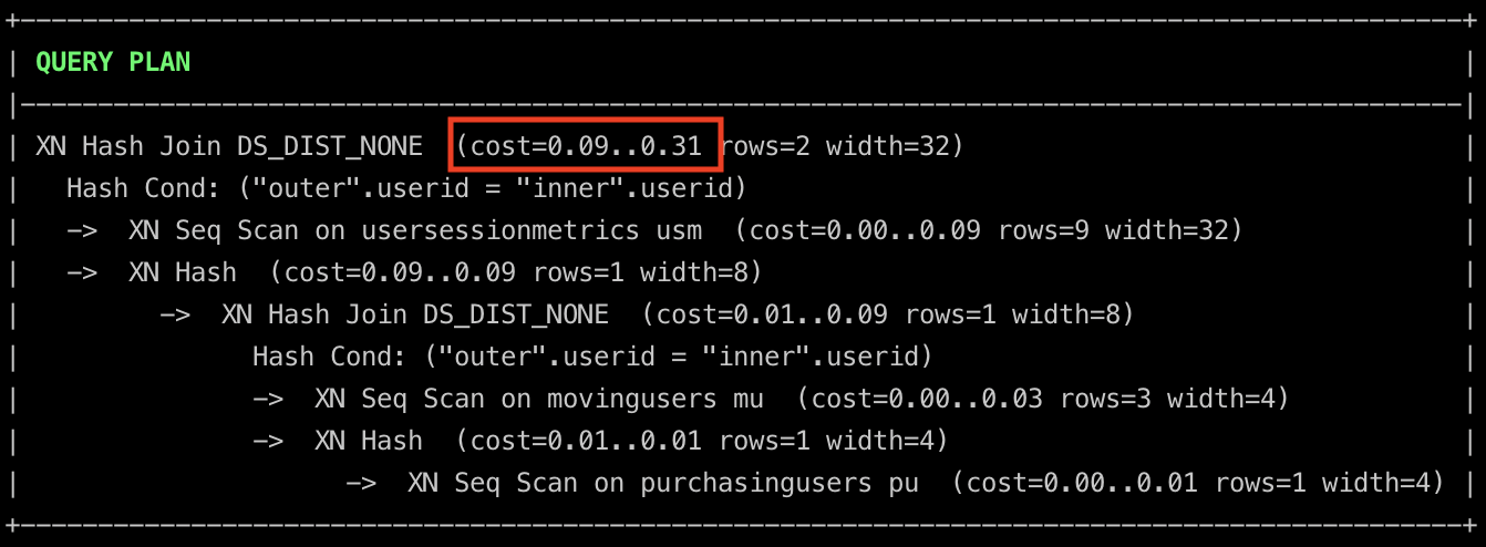
The cost is lower than the previous approaches. This is because the temporary tables required for the final selection have been precomputed. The generation of these temporary tables is not free. The cost of generating temporary tables is shown below.

purchasingUsers Cost 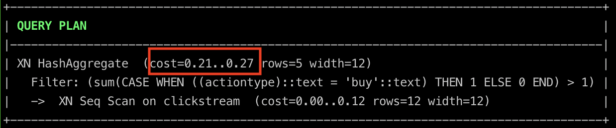tt 1 query plan

movingUsers Cost 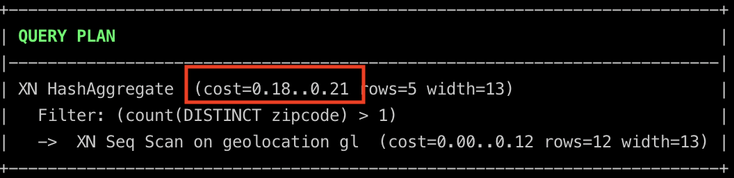tt 2 query plan

userSessionMetrics Cost 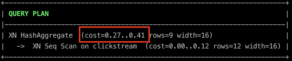tt 3 query plan

\q -- exit pgcli

Trade-offs

For most cases using CTEs or subquery or derived tables does not make a huge performance impact. The usual deciding factor is readability, which is a subjective measure. Also, note that CTEs performance is DB dependent.

If you are going to be reusing the temp tables in multiple queries it makes sense to calculate them once and reuse them.

Generally, it is good practice to always check the query plans for best performance. There is also a readability factor that is hard to be objective on. Some prefer CTEs as it makes understanding the query easier. But having a query with tens of CTEs might not be the best approach for readability.

Tear down

Delete AWS Redshift cluster, to prevent unnecessary costs.

aws redshift delete-cluster --cluster-identifier sdesamplecluster --skip-final-cluster-snapshot

Conclusion

To recap we saw

What Common Table Expressions(CTEs) are.
How to use them.
Performance trade-offs compared to the subquery, derived table, and temp table.
Readability.

Hope this article helps you understand CTEs in detail. The next time you come across a complex query try CTEs and see if you can improve readability.

References

Please consider sharing, it helps out a lot!