%%{init: {'theme': 'base', 'themeVariables': {'fontSize': '14px', 'fontFamily': 'arial'}}}%%
flowchart TD
    subgraph EXTRACT
        A{"Does source have created/updated_at time?"} -->|Yes| B["Extract data based on created/updated_at time"]
        A -->|No| C["Extract data based on diffs using primary key or md5 hash"]
    end
    B --> D["Transform data"]
    C --> D
    subgraph LOAD
        E{"Load data: Output data model?"}
        E -->|Fact| F["Overwrite partition"]
        E -->|SCD2| G["Merge into"]
        E -->|Duplicates acceptable: bronze layer | H["Append"]
        E -->|Transactional table| J["Delete & Upsert"]
        F --> I(["Done"])
        G --> I
        H --> I
        J --> I
    end
    D --> E

    classDef decision fill:#fff3cd,stroke:#d39e00,stroke-width:2px,color:#000
    classDef process fill:#d1ecf1,stroke:#0c5460,stroke-width:1px,color:#000
    classDef done fill:#d4edda,stroke:#155724,stroke-width:2px,color:#000

    class A,E decision
    class B,C,D,F,G,H,J process
    class I done

    style EXTRACT fill:#f8f9fa,stroke:#adb5bd,color:#000
    style LOAD fill:#f8f9fa,stroke:#adb5bd,color:#000
Introduction
Are you in a data (or data-adjacent) role and struggling with designing incremental loads? Do you struggle with
Identifying industry standard for large-scale data loads?
Structuring a data load pipeline for reliability & scalability?
Identifying which ingestion tools to use?
Then this post is for you.
With the right design, your large scale pipelines will just chug along.
By the end of this post, you will have a decision chart to design incremental data pipelines for your use case.
We use source and destination to refer to input and output table(s).
Video walkthrough
Source’s timestamp column dictates extraction logic
The three types of source columns which dictate extraction logic are:
Updated_at (timestamp): This column represents when a row was updated. If this column is available, use it to pull the incremental changes. Ensure that when a row is initially created, updated_at is set to inserted_at.Inserted_at (timestamp): This column represents when a row was inserted into source data. Use this column only if updated_at is unavailable. Usually, this case applies only to append-only sources, such as facts.No updated/inserted_at: In this case, we will need to compare the source and destination data to identify the differing rows. The difference can be identified by comparingprimary keys (PKs); if there’s no PK, construct one (e.g., md5 hash of the row).
Assuming we are pulling data from the source for a given time period: start_ts -> end_ts.
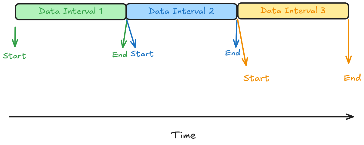
Let’s see the SQL for data extraction.
Select * From source
Where updated_at >= start_ts And updated_at < end_ts;
Select * From source
Where inserted_at >= start_ts And inserted_at < end_ts;
Select * From source
Where inserted_at > (select max(inserted_at) from destination);
Select s.* From source As s
Left Join destination As d On s.pk = d.pk
Where d.pk Is NULL;
Select s.* From source As s
Left Join
destination As d
On md5_hash(s.columns_that_make_up_pk) = md5_hash(d.columns_that_make_up_pk)
Where md5_hash(s.columns_that_make_up_pk) Is NULL;- 1
- Data with update_at (ts) in range
- 2
- Data with inserted_at (ts) in range
- 3
- Data after the most recent ETL into destination
- 4
- New data identified with primary key
- 5
- New data identified with hash of composite key (business knowledge)
Note
Same extract patterns apply to API data pulls.
There may be cases where 3rd-party data dumped into your S3/SFTP/FTP servers will need to be fully loaded before the data can be pulled.
But once loaded, the above patterns will apply.
Checkout this article that goes over how to use Airflow to define start and end times ->
Video walkthrough
Load strategy depends on destination data model
There are 3 main strategies to load data into our destination:
Overwrite partitions:- We replace entire data partitions for each pipeline run. The destination tables are partitioned by event time (created_at or updated_at).
- Gold standard for re-runnability without manual intervention. E.G., overwritePartitions.
- Common data models: Facts & Snapshot dimensions.
Row-based update/insert/delete:- We update/insert/delete rows identified by some id. Typical for SCD2 and updating destination tables.
- This also covers the
DELETE by rows & INSERTpattern - Inefficient and requires a clean-up step before re-runnability.
- Functions: MERGE INTO, INSERT ON CONFLICT, DELETE & INSERT etc
Append:- Append all the rows to the destination.
- This is typically done for data, where duplication is ok, or where we de-duplicate downstream.
- Typically done when ingesting high-velocity data from a stream.
- Tools like Kafka offer settings that let us append new data only to the destination (at atmost once link).
%%{init: {'theme': 'base', 'themeVariables': {'fontSize': '14px', 'fontFamily': 'arial'}}}%%
flowchart TB

    %% ===== PATTERN 1: OVERWRITE PARTITION =====
    subgraph P1["OVERWRITE PARTITION"]
        direction LR
        IN1["[D2]"] --> L1["LOAD"]
        L1 -->|"DELETE & INSERT"| DEST1
        subgraph DEST1["DESTINATION DATA, PARTITIONED BY DAY"]
            direction TB
            D1a["D1"] ~~~ D2old["D2"] ~~~ D2new["D2"] ~~~ D3a["D3"]
        end
    end

    %% ===== PATTERN 2: ROW BASED UPDATE/INSERT/DELETE =====
    subgraph P2["ROW BASED UPDATE / INSERT / DELETE"]
        direction LR
        IN2["[r1, r5, r10]"] --> L2["LOAD"]
        L2 --> DEST2
        subgraph DEST2["DESTINATION DATA"]
            direction TB
            R1["r1 — UPDATE"] ~~~ R5["r5 — DELETE"] ~~~ R10["r10 — INSERT"]
        end
    end

    %% ===== PATTERN 3: APPEND ONLY =====
    subgraph P3["APPEND ONLY"]
        direction LR
        IN3["[r1, r5, r10]"] --> L3["LOAD"]
        L3 --> DEST3
        subgraph DEST3["DESTINATION DATA"]
            direction TB
            E1["r1"] ~~~ E5["r5"] ~~~ A1["r1 (appended)"] ~~~ A5["r5 (appended)"] ~~~ A10["r10 (appended)"]
        end
    end

    %% ===== Force vertical order P1 -> P2 -> P3 =====
    P1 ~~~ P2 ~~~ P3

    %% ===== STYLING =====
    classDef load fill:#ffffff,stroke:#333,stroke-width:1px,color:#000
    classDef neutral fill:#ffffff,stroke:#333,stroke-width:1px,color:#000
    classDef del fill:#f8c4c4,stroke:#c0392b,stroke-width:1px,color:#000
    classDef ins fill:#bfe6c3,stroke:#27ae60,stroke-width:1px,color:#000
    classDef upd fill:#aed6f1,stroke:#2980b9,stroke-width:1px,color:#000

    class L1,L2,L3 load
    class D1a,D3a,E1,E5 neutral
    class D2old,R5 del
    class D2new,R10,A1,A5,A10 ins
    class R1 upd

    style IN1 fill:#ffffff,stroke:#ffffff,color:#000
    style IN2 fill:#ffffff,stroke:#ffffff,color:#000
    style IN3 fill:#ffffff,stroke:#ffffff,color:#000
    style P1 fill:#f8f9fa,stroke:#adb5bd,color:#000
    style P2 fill:#f8f9fa,stroke:#adb5bd,color:#000
    style P3 fill:#f8f9fa,stroke:#adb5bd,color:#000
    style DEST1 fill:#ffffff,stroke:#999,color:#000
    style DEST2 fill:#ffffff,stroke:#999,color:#000
    style DEST3 fill:#ffffff,stroke:#999,color:#000
Video walkthrough
Design pipelines for easy backfilling
Backfills are inevitable. Make sure that they can be run without manual intervention (as much as possible).
If your pipelines depend on the destination data in any way, you need to clean up the destination before backfills.
# Does the destination require manual cleanup before backfill?
Extract logic: `Select * From Source
Where inserted_at > (Select max(inserted_at) From Destination)`
> Hint: The Extract logic depends on destination, so it needs to be cleaned.
1. [x] Yes
2. [ ] No
If a load step uses Update or Deletes, they require destination cleanup before backfills.
Running a backfill is the same as running the pipeline, but for a time range in the past.
Depending on data size and load logic, we need to trigger backfills in different ways.
Here are the 3 main scaling strategies for backfills (from easiest to complex options)
- Run the
backfill as a single process. We need sufficient resources to process the full range of data for backfilling. Serial pipeline runs. Most orchestrators support this. But our pipeline can be perpetually caught up in a state of catching up. For example, backfilling a 12 h run-time daily pipeline for 2 years will take a year to catch up to today.Parallel pipeline runs. Only possible if the runs are independent. i.e., destination should not be used in load and no-lookback-type calculations.
We can also combine 1 with 2 or 3, depending on resource availability, data size, and timelines to complete backfills.
flowchart TD
    Start([Start]) --> Q1{Enough resources to<br/>process full range<br/>in one go?}

    Q1 -->|Yes| S1[Strategy 1:<br/>Single Process]
    S1 --> S1a[Run backfill as one process<br/>over the full data range]
    S1a --> S1b[/Simplest option<br/>Requires sufficient resources/]

    Q1 -->|No| Q2{Are runs<br/>independent?}

    Q2 -->|No| S2[Strategy 2:<br/>Serial Pipeline Runs]
    S2 --> S2a[Run pipeline sequentially]
    S2a --> S2b[/Risk: perpetual catch-up<br/>e.g. 12h daily run x 2 yrs<br/>takes ~1 year to catch up/]

    Q2 -->|Yes| S3[Strategy 3:<br/>Parallel Pipeline Runs]
    S3 --> S3a[Run independent intervals<br/>concurrently]
    S3a --> S3b[/Fastest option<br/>Only valid when runs<br/>are fully independent/]
Bootstrap is the process of running a pipeline for all history till today, after which the pipeline runs incrementally. It is a special case of backfilling.
Note
It’s almost always recommended to bootstrap for the first run, and the following pipelines are run incrementally.
Video walkthrough
Additive schema changes are usually ok
Additive schema changes are when column data types are expanded (int → long) or when new columns are added.
If you have schema evolution, you can use it to handle schema evolution.
However, column meaning changes need manual intervention.
Conclusion
To recap, we saw
Incremental loading strategy depends on the nature of the source and the model of your destination tables.
Was this helpful? If yes, share it with a colleague who is designing incremental pipelines 🔗