How to quickly deliver data to business users? #1. Adv Data types & Schema evolution

• 1. Introduction
  • 1.1. Pre-requisites
• 2. Use Schema evolution & advanced data types to quickly deliver new columns to the end-user
  • 2.1. Enable schema evolution for additive column changes
  • 2.2. Model 1:1 relationship as STRUCT and 1:M relationships as ARRAY[STRUCTS] to keep schema changes self contained
  • 2.3. Naming conventions should represent relationship
• 3. Create systems to effectively leverage schema evolution
  • 3.1. Auto schema evolution is high-risk & high-reward, don’t use it for sensitive data
  • 3.2. Validate relationships before processing data to avoid presenting bad data to end-users
  • 3.3. Be careful when you explode and aggregate to avoid multiple counting
  • 3.4. Manually validate new data before exposing it to end-user
  • 3.5. Use a view interface for nontechnical stakeholders
  • 3.6. Limit relationship depth to 1
• 4. Conclusion
• 5. Recommended reading

1. Introduction

Over the past decade, every department has wanted to be data-driven, and data engineering teams are under more pressure than ever.

If you have been an engineer for over a few years, you would have seen your world change from a “well-planned data model” to a “dump everything in S3 and get some data for the end-user”.

Data engineers are under a lot of stress caused by :

The Business is becoming too complex, and every department wants to become data-driven; thus, expectations from the data teams skyrocket.

Not having enough time to pay down tech debt or spend time properly modeling the data required

Businesses act like they do not have the time/money, or patience to spend time doing things the right way.

Too many requirements with too many stakeholders

If so, this post is for you. Imagine building systems enabling you to deliver any new data stakeholders want in minutes. You will be known for delivering quickly and empowering the business to make more money.

This post will discuss an approach to quickly delivering new data to your end user. By the end of this post, you will have a technique to apply to your pipelines to make your life easier and boost your career.

1.1. Pre-requisites

The techniques you will learn in this post apply to any pipeline. In the code example, we will follow.

1. 3-hop architecture: Data is transformed in pre-defined ways as it flows through the layers:
   1. Raw: A data dump from the upstream sources as is.
   2. Bronze: The raw data’s data types and column names are changed to match the warehouse standards.
   3. Silver: This layer involves modeling bronze data based on one of Kimball, Data vault, etc.
   4. Gold: This layer involved modeling data for end-user consumption. We can further split this layer into 2: OBT: Fact tables with all their dimensions left joined to them and pre_agg_* tables, which are end-user-specific tables built from the OBT tables.
   5. Read this for a detailed introduction to the 3-hop architecture .
2. Apache Spark and Apache Iceberg: We will use Spark and Iceberg to demonstrate advanced data types and schema evolution. Read this for a quick introduction to Apache Iceberg .

The code for this post and setup instructions are available here .

2. Use Schema evolution & advanced data types to quickly deliver new columns to the end-user

A data engineer’s job is to ensure that stakeholders can effectively use data to make decisions. A big part of DE work is getting new columns to your end users.

Build systems that automate adding new columns and making them available for the end-user.

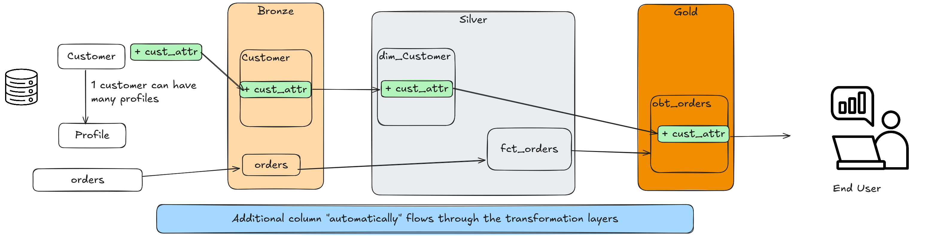
In this post we will use the following data flow to explain how to add new columns automatically to your datasets.

1. A customer can have multiple profiles.
2. An order is made by a customer.
3. We will combine customer + profile -> dim_customer.
4. We will combine fct_orders + dim_customer -> obt_orders.

2.1. Enable schema evolution for additive column changes

TL;DR: Use schema evolution to add new columns or expand existing ones without a data engineer having to add the columns manually.

Most modern table formats enable schema evolution.

We create iceberg tables that are receptive to schema changes automatically, as follows:

TBLPROPERTIES (
    'format-version' = '2',
    'write.spark.accept-any-schema'='true'
);

The write.spark.accept-any-schema setting needs to be set on the table to enable any system writing to it to be able to add new columns that are not present in the table schema (reference docs ).

Let’s see how this works in the code

# Code to load data into obt_orders table
def transform(self, input_dfs):
    print("Starting TRANSFORM...")
    fct_orders = input_dfs.get("fct_orders")
    dim_customer = input_dfs.get("dim_customer")

    order_cols = fct_orders.columns
    dim_customer_cols = dim_customer.columns
    
    return fct_orders.join(
        dim_customer,
        on="customer_id"
    ).select(
        *
        , F.struct(
            *[dim_customer[dim_customer_col] for dim_customer_col in dim_customer_cols]
        ).alias("customer")
    ).drop("customer_id")

def load(self, transformed_df):
    print("Starting LOAD...")
    transformed_df = transformed_df.withColumn("etl_upserted", F.current_timestamp())
    transformed_df\
    .writeTo("prod.db.obt_orders")\
    .option("check-ordering", "false")\
    .option("mergeSchema", "true")\
    .overwritePartitions()

From the above code, we see:

1. Use a select * in the join logic to ensure that every column is selected. While typically a bad practice, the select * here provides us with all the columns of the source data.
2. All of the columns from dim_customer modeled as a STRUCT.
3. When writing data into the table, we use the mergeSchema=true option to enable spark to write a dataframe with mismatched schema into this iceberg table (reference docs ).
4. check-ordering=false to ensure that the column order of the dataframe need not match the column order of the table’s schema.

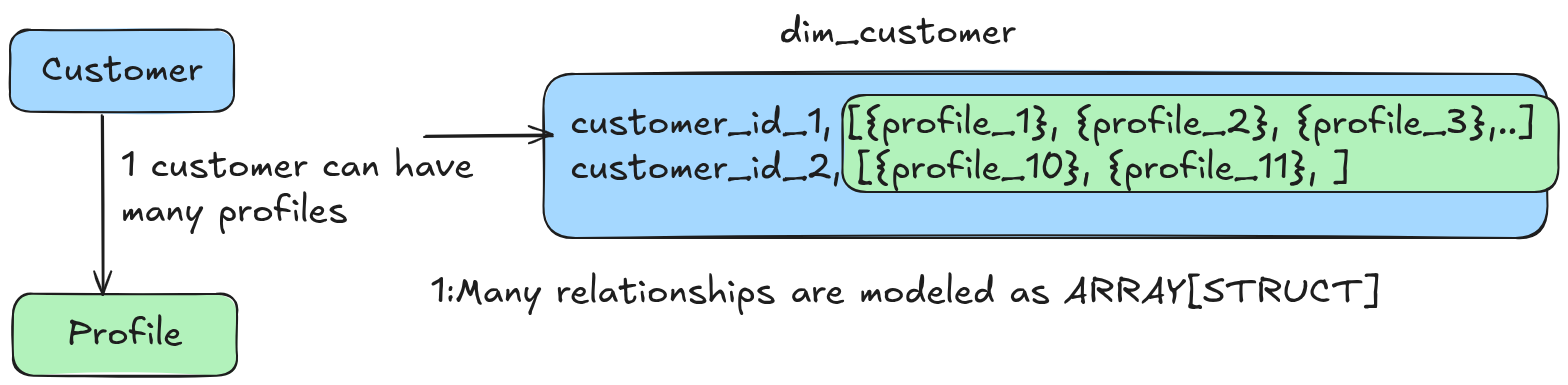
2.2. Model 1:1 relationship as STRUCT and 1:M relationships as ARRAY[STRUCTS] to keep schema changes self contained

TL;DR:

1. 1:1 relationships -> Model one table as a STRUCT column in the other table’s dimension.
2. 1:M relationships -> Model the M table as an ARRAY[STRUCT] column in the 1 table’s dimension
3. Do not model a fact inside a dimension table.

Read this article for a detailed explanation of using advanced data types

Datasets are usually related to each other in one of 3 ways:

1. 1:M: One row in a table can be related to M rows in another. For example, one customer can have multiple profiles. In this case, the profile will be an ARRAY[STRUCT] in the customer dimension.
2. 1:1: One row in a table can be related to another row in another. For example, one customer can have one active address, which will be a STRUCT column in the customer dimension.
3. M:M: Multiple rows in a table can be related to multiple rows in another. For example, multiple orders can have various items, and multiple items can be part of various orders. M:M relationships are tricky to model with advanced data types, as they can lead to circular dependency. The simplest way to solve this is to have a bridge_table and keep the entities as separate tables.

Note that the relationships are one-way. For example, one customer is related to many profiles, but the other way is not a 1:M relationship.

Modeling data as STRUCTS and ARRAY[STRUCT] with schema evolution enables us to add new columns without managing the table schemas.

When you get a new column in an upstream table, your logic will inherit the same name but place it inside the STRUCT.

2.3. Naming conventions should represent relationship

TL;DR Use singular column name for STRUCT and plural for ARRAY[STRUCT]. The naming convention should represent the entity’s relationship.

Accessing columns with the . function is intuitive compared to a DE having to name every column. For example, the column name customer.datetime_update indicates that the column belongs to the customer entity.

Our customer and profile upstream tables have the datetime_updated column in our example.

However, since the product information is within a STRUCT, we can use the same name for it.

If we hadn’t used a STRUCT, we would have had to deal with columns of the same name.

select order_id
, order_date
, customer.customer_id
, customer.first_name
, customer_profiles.profile_id
, customer_profiles.profile_name
, customer_profiles.profile_type
, customer_profiles.datetime_created -- We can clearly tell which datetime_created corresponds to profiles and customer
, customer.datetime_created
from prod.db.obt_orders 
LATERAL VIEW EXPLODE(customer.profiles) as customer_profiles

From the above, we see that the schema represents the relationships.

3. Create systems to effectively leverage schema evolution

Pipelines that change the structure of data have the potential to break downstream consumers. We need to monitor the pipelines and have systems in place to debug and fix issues promptly.

3.1. Auto schema evolution is high-risk & high-reward, don’t use it for sensitive data

Automatic schema evolution is a high-risk pattern since you are essentially trying to automate parts of data context and understanding (which is key for data modeling). As such, a bug can change the meaning of the data.

For example, if upstream changes the relationship of order -> customer and allows profiles to make an order, the above pipeline will start having no customer profiles. Or if the upstream team decides to create an additional join key to join customers to profiles, your pipeline will not catch it before causing damage.

Due to potential issues, it is advisable not to use this pattern for highly sensitive data such as finance, PII, etc.

3.2. Validate relationships before processing data to avoid presenting bad data to end-users

The above approach depends on the relationship between entities holding. If the upstream table relationships change, the pipeline will fail. To avoid this, we should have input validation that checks if the relationship holds.

If your fact table that has a customer_id decides that each order will now record the profile id, you would need to update your pipeline logic.

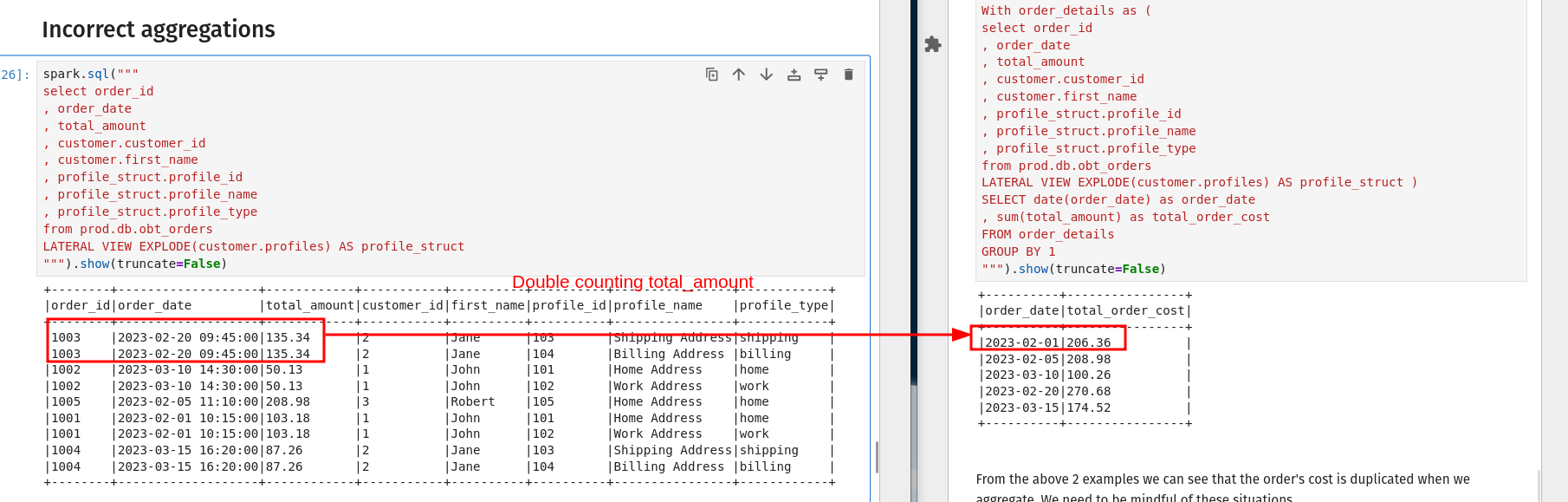
3.3. Be careful when you explode and aggregate to avoid multiple counting

With the standard fact and dimensional model, you’d always ensure one row per grain in the fact table before aggregating. When using an ARRAY[STRUCT], you need to be careful when you aggregate data so that you don’t count rows multiple times.

If you want to see the average order cost per profile per day, it’s not a simple group by + avg; you have to define how the cost of an order can be attributed to a profile.

1. Do you split the cost evenly across profiles? or
2. Do you assign the exact total order cost to each profile? or
3. Do you use some algorithm to attribute cost to the profile you think is the purchaser? or
4. The best option is to have the order system record the profile ID along with the customer ID as part of the order.

3.4. Manually validate new data before exposing it to end-user

While the data may flow into your gold OBT layers, you should ensure that it is ready for the end user with care. The key idea is that your OBT powers data marts.

Having the data shouldn’t mean exposing it to the end user without consideration. The person building the data mart should always validate the data before exposing it to the end user.

3.5. Use a view interface for nontechnical stakeholders

Most end users of your data may not be aware of advanced data types or that table schema can evolve rapidly. If your end users fall into this category, then it is hugely beneficial to have a view in front of your OBT table to enable easy consumption.

You can split out the array or struct into a schema suitable for the end user. With this view, the end user, who may be used to a traditional data model, may access the data, reducing the possibility of making mistakes.

Note: Keep view logic light as it can be expensive to do EXPLODE for each query

3.6. Limit relationship depth to 1

When you build ARRAY[STRUCTS], it is tempting to build ARRAY[STRUCT[ARRAY[STUCTS]S]] and so on. While this approach may seem intuitive, it can cause a lot of issues with how the table is used, such as

1. Multiple EXPLODE making usage slow and code error-prone
2. Costs. The ARRAY[STRUCT] approach takes advantage of our cheap storage. However, if we are not mindful of the levels of nesting, we may cause the cost to skyrocket.

4. Conclusion

To recap we saw

1. How to use advanced data types and schema evolution to automate adding new columns
2. How auto schema evolution is a high-risk high-reward approach and its caveats
3. How to enable non technical users with a view interface for data access

The next time you realize that you are spending a lot of time adding new columns to existing dataset, use this approach to move faster. Your end-users and manager will thank you.

Please let me know in the comment section below if you have any questions or comments.

5. Recommended reading

1. Multi-hop architecture
2. Table formats and their benefits
3. Data quality checks

If you found this article helpful, share it with a friend or colleague using one of the socials below!