Data Engineering Project for Beginners - Batch edition
- Introduction
- Approach
- Project overview
- Engineering Design
- Setup
- Code and explanation
- Monitoring ETL
- Design Review
- Common Scenarios
- Next Steps
- Conclusion
Introduction
Starting out in data engineering can be a little intimidating, especially because data engineering involves a lot of moving parts. I have seen and been asked questions like
I’m a data analyst who is striving to become a data engineer. What are some
awsproject ideas that I could start working on and gain some DE experience?
Are there any front-to-back tutorials for a basic DE project?
What is a good project to get DE experience for job interviews?
The objective of this article is to help you
-
Build and understand a data processing framework used for Batch data loading by companies
-
Set up and understand the cloud components involved (Redshift, EMR)
-
Understand how to spot failure points in an data processing pipeline and how to build systems resistant to failures and errors
-
Understand how to approach or build an data processing pipeline from the ground up
Approach
The best way to get a good understanding of any topic is to try it out and build something with it. Following this approach, to understand building an data processing pipeline we will build our own. Based on data from open data sources such as uci and kaggle that have been modified a little to enable joins.
Project overview
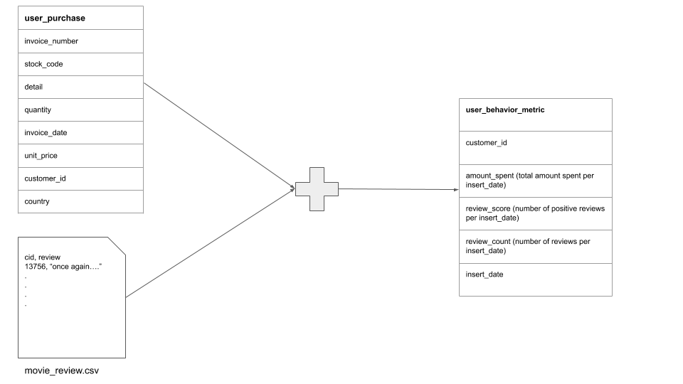
For our project we will assume we work for a user behavior analytics company that collects user data from different data sources and joins them together to get a broader understanding of the customer. For this project we will consider 2 sources,
Purchase datafrom an OLTP databaseMovie review datafrom a 3rd party data vendor (we simulate this by using a file and assuming its from a data vendor)
The goal is to provide a joined dataset of the 2 datasets above, in our analytics (OLAP) database every day, to be used by analysts, dashboard software, etc.
Engineering Design
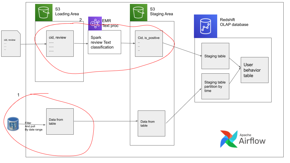
We use a standard load-stage-clean pattern for storing out data. We will also design our ETL with idempotent functions, for cleaner reruns and backfills.
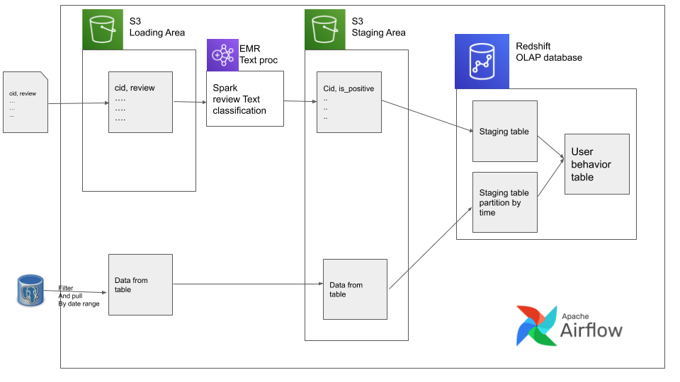
NOTE: we don’t need Redshift or EMR in our data pipeline, since the data is very small in our example. But we use it to “simulate” a real big data scenario.
Airflow Primer:
Airflow runs data pipelines using DAG’s. Each DAG is made up of one or more tasks which can be stringed to gether to get the required data flow. Airflow also enables templating, where text surrounded by {{ }} can be replaced by variables when the DAG is run. These variables can either be passed in by the user as params, or we can use inbuilt macros
for commonly used variables. Airflow runs DAG’s based on time ranges, so if you are running a DAG every day, then for the run happening today, the execution day of airflow will be the yesterday, because Airflow looks for data that was created in the previous time chunk(in our case yesterday).
Setup
From the above engineering spec you can see that this is a fairly involved project, we will use the following tools
- docker
(also make sure you have
docker-compose) we will use this to run Airflow locally - pgcli to connect to our databases(postgres and Redshift)
- AWS account to set up required cloud services
- AWS Components to start the required services
By the end of the setup you should have(or know how to get)
aws cliconfigured with keys and regionpem or ppkfile saved locally with correct permissionsARNfrom youriamrole for RedshiftS3bucketEMR IDfrom the summary pageRedshifthost, port, database, username, password and have the appropriateiamrole associated with it for runningSpectrumqueries.
NOTE We try to keep the cost very low, and it will be given that we are dealing with small data for our example, but it will still cost some money. Please switch on only while using and don’t forget to switch it off after use.
Code and explanation
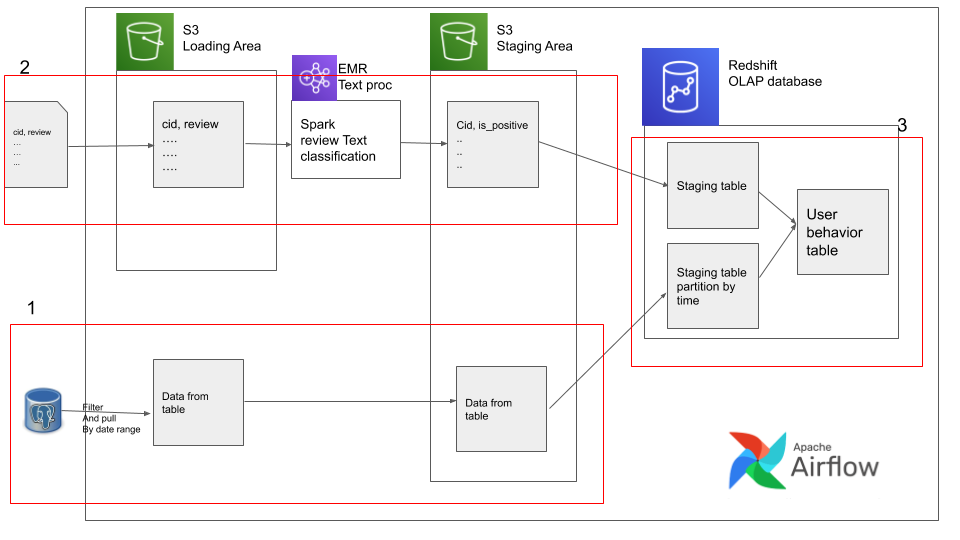
For ease of implementation and testing, we will build our data pipeline in stages. There are 3 stages and these 3 stages shown below
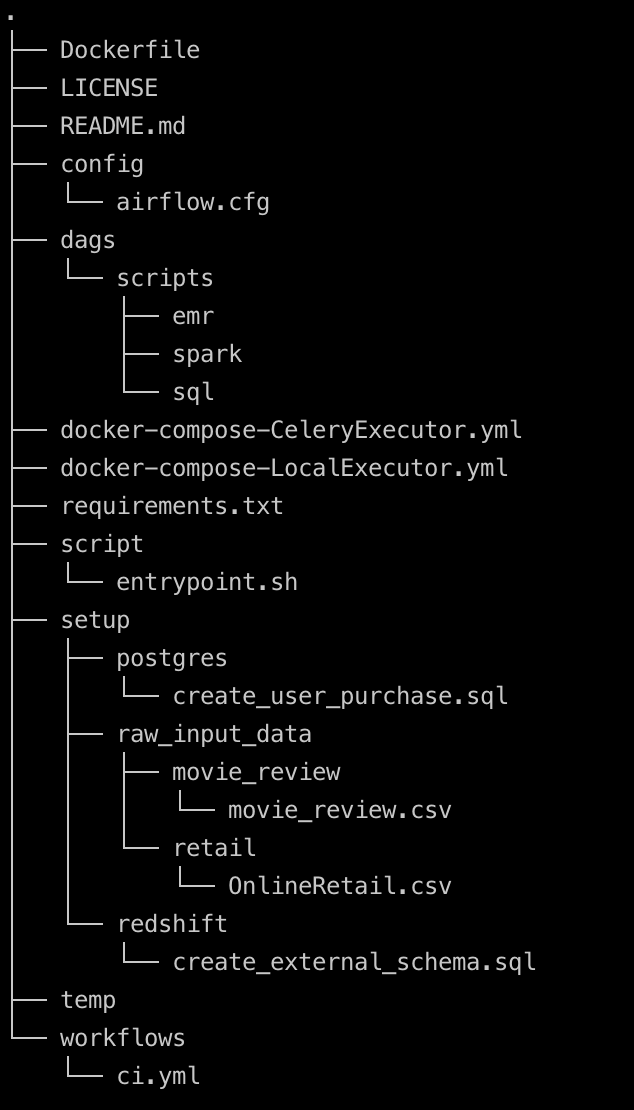
In order to get started git clone this git repo
and work of the starter branch(git checkout starter). This is the airflow docker implementation forked from the popular puckle airflow
docker image with some additional changes for our data pipeline.
We will work on one stage(from the above diagram) at a time.
Stage 1. pg -> file -> s3
cd to your airflow repository and start up the docker services using the compose file a shown below
docker-compose -f docker-compose-LocalExecutor.yml up -d
This command starts the airflow webserver and postgres database for metadata. You can verify that the docker containers have started using docker ps
Download the data required for using the following link
Place this in /beginner_de_project/setup/ location.
Your project directory should look like
Since we are not dealing with a lot of data we can use or Airflow metadata database as our “fake” datastore as well. Open a connection to pg database using pgcli as shown below
pgcli -h localhost -p 5432 -U airflow -d airflow
# the password is also airflow
Let’s set up our fake datastore. In your pgcli session run the following script
CREATE SCHEMA retail;

CREATE TABLE retail.user_purchase (
    invoice_number varchar(10),
    stock_code varchar(20),
    detail varchar(1000),
    quantity int,
    invoice_date timestamp,
    unit_price Numeric(8,3),
    customer_id int,
    country varchar(20)
);

COPY retail.user_purchase(invoice_number,
stock_code,detail,quantity,
invoice_date,unit_price,customer_id,country)
FROM '/data/retail/OnlineRetail.csv'
DELIMITER ','  CSV HEADER;
This is also available in your repo at setup/postgres/create_user_purchase.sql. This script creates the source table and loads in the data. Do a count(*) on the user_purchase table, there should be 541908 rows.
Now we are ready to start writing our data pipeline. Let’s create our first airflow dag in the dags folder and call it user_behaviour.py. In this script lets create a simple Airflow DAG as shown below
from datetime import datetime, timedelta
from airflow import DAG
from airflow.operators.dummy_operator import DummyOperator
default_args = {
"owner": "airflow",
"depends_on_past": True,
'wait_for_downstream': True,
"start_date": datetime(2010, 12, 1), # we start at this date to be consistent with the dataset we have and airflow will catchup
"email": ["airflow@airflow.com"],
"email_on_failure": False,
"email_on_retry": False,
"retries": 1,
"retry_delay": timedelta(minutes=5)
}
dag = DAG("user_behaviour", default_args=default_args,
schedule_interval="0 0 * * *", max_active_runs=1)
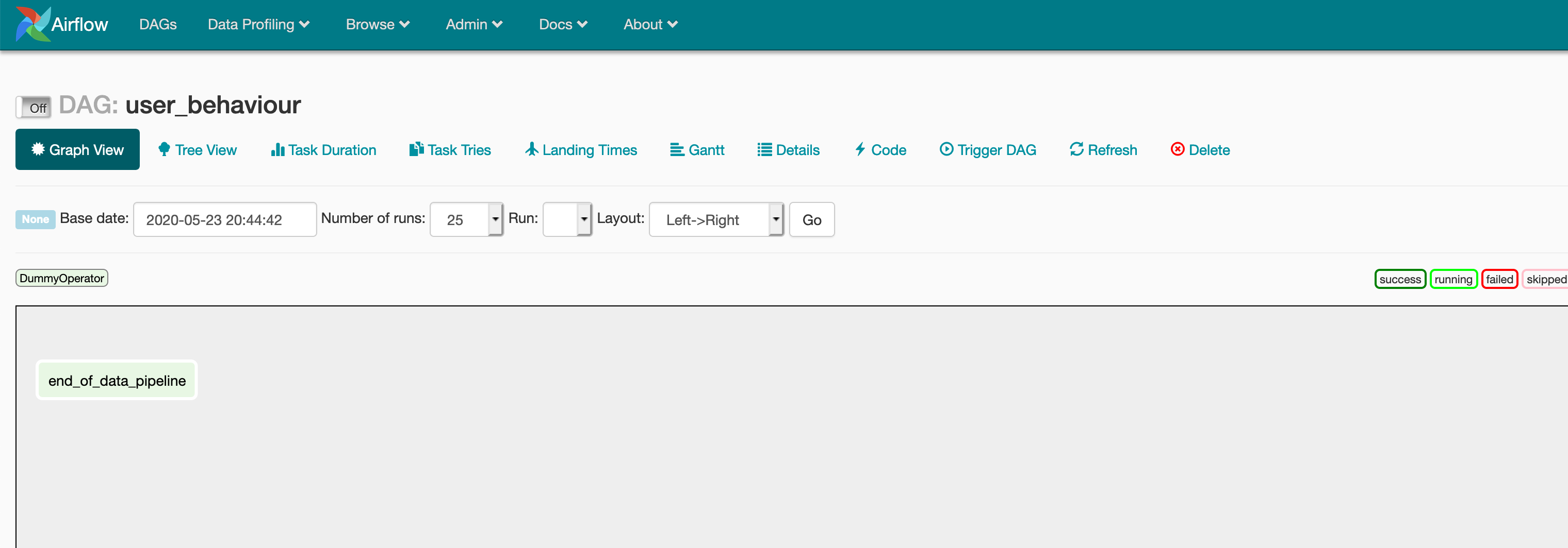
end_of_data_pipeline = DummyOperator(task_id='end_of_data_pipeline', dag=dag)
end_of_data_pipeline
This DAG basically does nothing but runs a dummy operator (which does nothing). If you go to http://localhost:8080 you will be able to see the airflow UI up. If you are using windows you may need to follow https://github.com/puckel/docker-airflow/issues/312#issuecomment-497408401 to get you host ip. You should be able to see something like shown below
Now let’s build up on what we already have and unload data from pg into a local file. We have to unload data for the specified execution day and only if the quantity is greater than 2. Create a script called filter_unload_user_purchase.sql in the /dags/scripts/sql/ directory
COPY (
    select invoice_number,
           stock_code,
           detail,
           quantity,
           invoice_date,
           unit_price,
           customer_id,
           country
      from retail.user_purchase
     where quantity > 2
       and cast(invoice_date as date)='{{ ds }}')
TO '{{ params.temp_filtered_user_purchase }}' WITH (FORMAT CSV, HEADER);
In this templated SQL script we use {{ ds }} which is one of airflow’s inbuilt macros to get the execution date. {{ params.temp_filtered_user_purchase }} is a parameter we have to set at the DAG. In the DAG we will use a PostgresOperator to execute the filter_unload_user_purchase.sql sql script. Add the following snippet to your DAG at user_behaviour.py.
# existing imports
from airflow.operators.postgres_operator import PostgresOperator

# config
# local
unload_user_purchase ='./scripts/sql/filter_unload_user_purchase.sql'
temp_filtered_user_purchase = '/temp/temp_filtered_user_purchase.csv'
# existing code

pg_unload = PostgresOperator(
    dag=dag,
    task_id='pg_unload',
    sql=unload_user_purchase,
    postgres_conn_id='postgres_default',
    params={'temp_filtered_user_purchase': temp_filtered_user_purchase},
    depends_on_past=True,
    wait_for_downstream=True
)

pg_unload >> end_of_data_pipeline
Your diff should be similar to one as shown below
from datetime import datetime, timedelta

from airflow import DAG
from airflow.operators.dummy_operator import DummyOperator
++from airflow.operators.postgres_operator import PostgresOperator


++# config
++# local
++unload_user_purchase ='./scripts/sql/filter_unload_user_purchase.sql'
++temp_filtered_user_purchase = '/temp/temp_filtered_user_purchase.csv'

default_args = {
    "owner": "airflow",
    "depends_on_past": False,
    "start_date": datetime(2010, 12, 1),
    "email": ["airflow@airflow.com"],
    "email_on_failure": False,
    "email_on_retry": False,
    "retries": 1,
    "retry_delay": timedelta(minutes=5)
}

dag = DAG("user_behaviour", default_args=default_args,
          schedule_interval="0 0 * * *")

end_of_data_pipeline = DummyOperator(task_id='end_of_data_pipeline', dag=dag)

++pg_unload = PostgresOperator(
++    dag=dag,
++    task_id='pg_unload',
++    sql=unload_user_purchase,
++    postgres_conn_id='postgres_default',
++    params={'temp_filtered_user_purchase': temp_filtered_user_purchase},
++  depends_on_past=True,
++ wait_for_downstream=True
++)

-- end_of_data_pipeline
++pg_unload >> end_of_data_pipeline
Ideally you will have your configs in a different file or set them as docker env variables, but due to this being a simple example we keep them with the DAG script.
You can verify that your code is working by going to the airflow UI at localhost:8080 and clicking on the dag and task and render as shown below
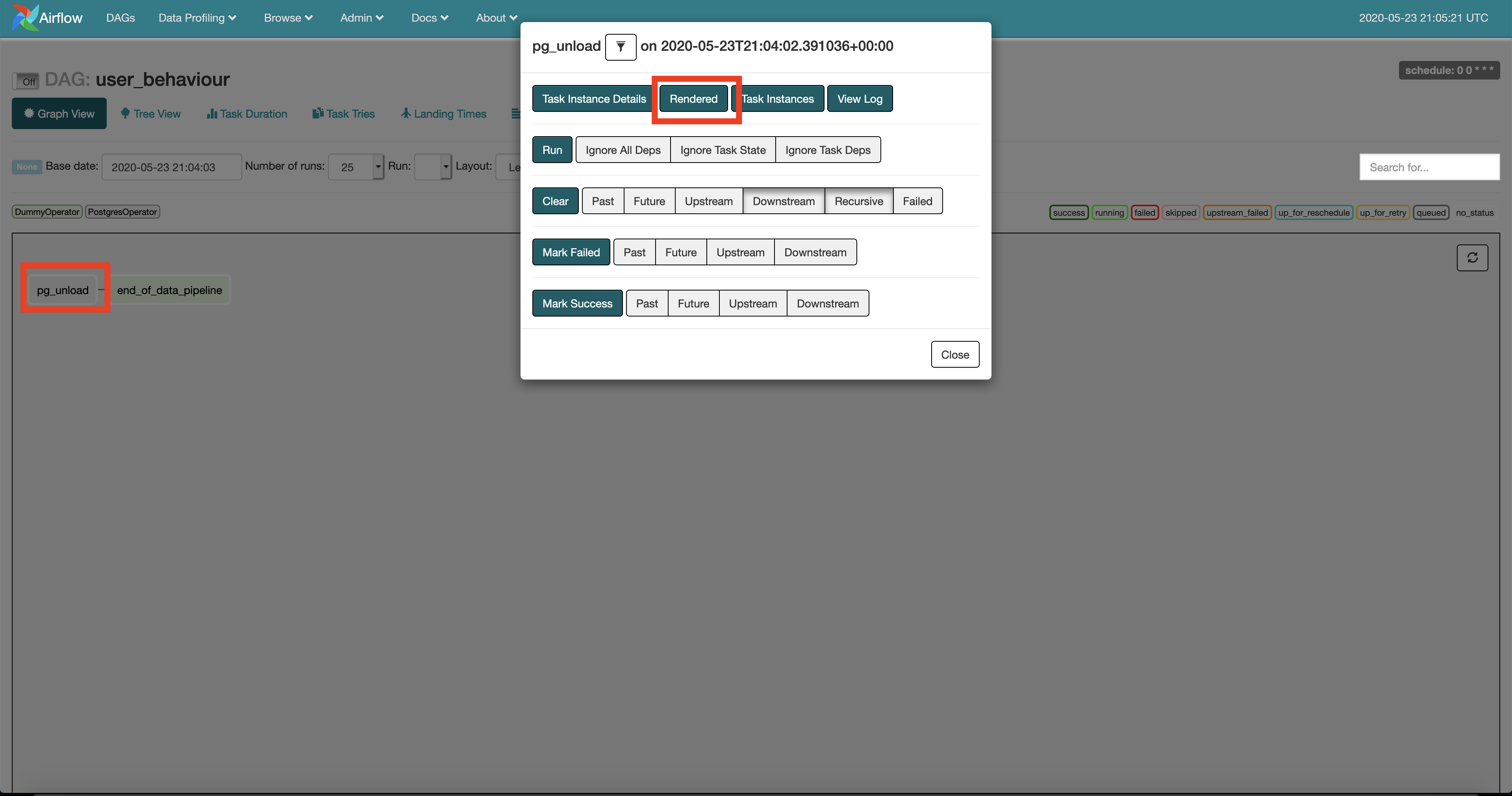
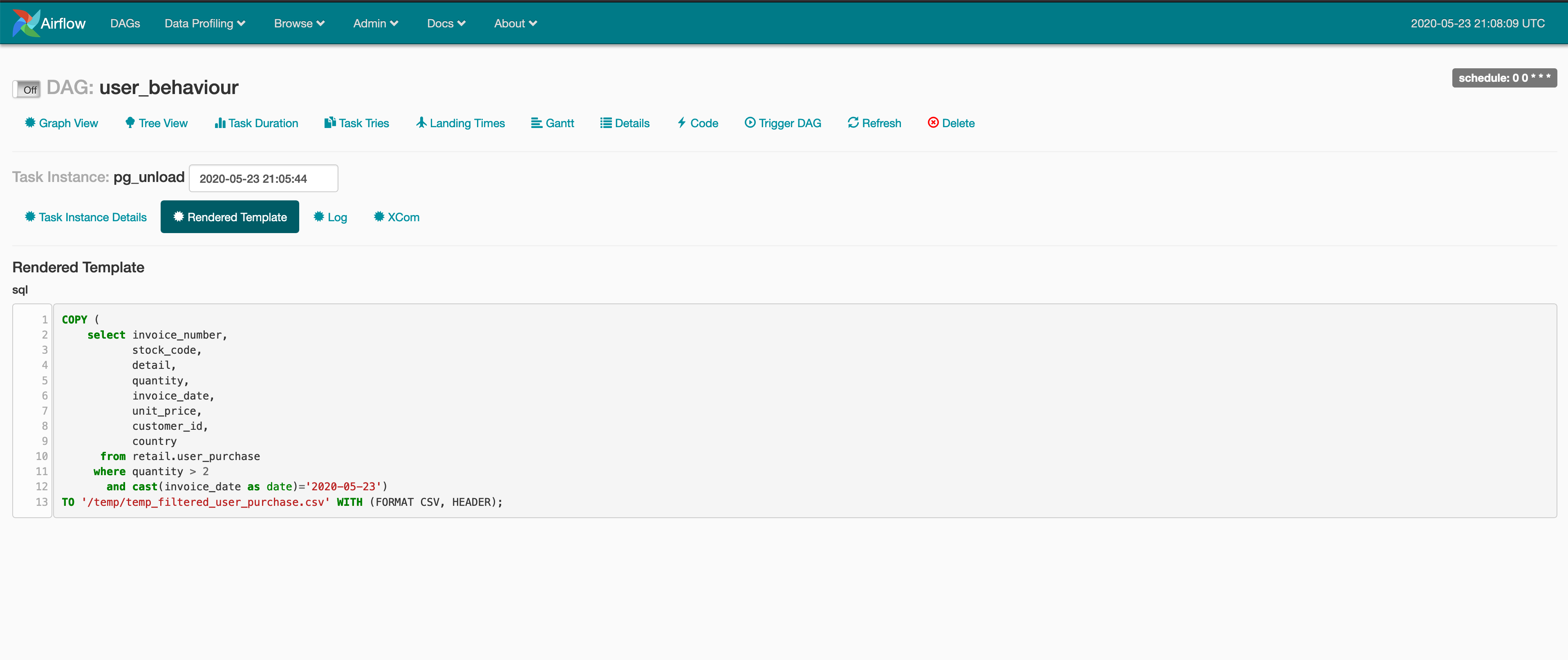
You will see that the {{ }} template in your SQL script will have been replaced by parameters set in the DAG at user_behaviour.py.
For the next task lets upload this file to our S3 bucket.
# existing imports
from airflow.hooks.S3_hook import S3Hook
from airflow.operators import PythonOperator

# existing config
# remote config
BUCKET_NAME = '<your-bucket-name>'
temp_filtered_user_purchase_key= 'user_purchase/stage/{{ ds }}/temp_filtered_user_purchase.csv'

# helper function(s)

def _local_to_s3(filename, key, bucket_name=BUCKET_NAME):
    s3 = S3Hook()
    s3.load_file(filename=filename, bucket_name=bucket_name,
                 replace=True, key=key)

# existing code
user_purchase_to_s3_stage = PythonOperator(
    dag=dag,
    task_id='user_purchase_to_s3_stage',
    python_callable=_local_to_s3,
    op_kwargs={
        'filename': temp_filtered_user_purchase,
        'key': temp_filtered_user_purchase_key,
    },
)

pg_unload >> user_purchase_to_s3_stage >> end_of_data_pipeline
In the above snippet we have introduced 2 new concepts the S3Hook and PythonOperator. The hook is a mechanism used by airflow to establish connections to other systems(S3 in our case), we wrap the creation of an S3Hook and moving a file from our local filesystem to S3 using a python function called _local_to_s3 and call it using the PythonOperator.
Once the data gets uploaded to S3 we should remove it from our local file system to prevent wasting disk space on stale data. Let’s add another task to our DAG to remove this temp file.
import os
# existing imports

# existing helper function(s)
def remove_local_file(filelocation):
    if os.path.isfile(filelocation):
        os.remove(filelocation)
    else:
        logging.info(f'File {filelocation} not found')

# existing code
remove_local_user_purchase_file = PythonOperator(
    dag=dag,
    task_id='remove_local_user_purchase_file',
    python_callable=remove_local_file,
    op_kwargs={
        'filelocation': temp_filtered_user_purchase,
    },
)

pg_unload >> user_purchase_to_s3_stage >> remove_local_user_purchase_file >> end_of_data_pipeline
Now that we have completed the first stage(Stage 1. pg -> file -> s3), let’s do a test run. Go to the Airflow UI at http://localhost:8080 and switch on the DAG. Your DAG will start running and catching up, you should see your DAG running.
You can always reset the local airflow instance by running the following commands
docker-compose -f docker-compose-LocalExecutor.yml down
docker-compose -f docker-compose-LocalExecutor.yml up -d
pgcli -h localhost -p 5432 -U airflow
# and rerunning the query at setup/postgres/create_user_purchase.sql to reload data into pg
Stage 2. file -> s3 -> EMR -> s3
In this stage we assume we are getting a movie review data feed from a data vendor. usually the data vendor drops data in S3 or some SFTP server, but in our example let’s assume the data is available at setup/raw_input_data/movie_review/movie_review.csv
Moving the movie_review.csv file to S3 is similar to the tasks we did in stage 1
#config
# local
# existing local config
movie_review_local = '/data/movie_review/movie_review.csv' # location of movie review withing docker see docker-compose volume mount

# existing remote config
movie_review_load = 'movie_review/load/movie.csv'
# existing code


movie_review_to_s3_stage = PythonOperator(
    dag=dag,
    task_id='movie_review_to_s3_stage',
    python_callable=_local_to_s3,
    op_kwargs={
        'filename': movie_review_local,
        'key': movie_review_load,
    },
)

# existing data pipeline
movie_review_to_s3_stage
It’s similar to the previous task,but not directly dependent on any other task.
In EMR we have a feature called steps which can be used to run commands on the EMR cluster one at at time, we will use these steps to
-
Pull data from
movie_review_loadS3 location to EMR clusters HDFS location. -
Perform text data cleaning and naive text classification using a pyspark script and write the output to HDFS in the EMR cluster.
-
Push data from HDFS to a staging S3 location.
we can define the EMR steps as a json file, create a file beginner_de_project/dags/scripts/emr/clean_movie_review.json. Its content should be as follows
[
  {
    "Name": "Move raw data from S3 to HDFS",
    "ActionOnFailure": "CANCEL_AND_WAIT",
    "HadoopJarStep": {
      "Jar": "command-runner.jar",
      "Args": [
        "s3-dist-cp",
        "--src=s3://{{ params.BUCKET_NAME }}/{{ params.movie_review_load }}",
        "--dest=/movie"
      ]
    }
  },
  {
    "Name": "Classify movie reviews",
    "ActionOnFailure": "CANCEL_AND_WAIT",
    "HadoopJarStep": {
      "Jar": "command-runner.jar",
      "Args": [
        "spark-submit",
        "s3://{{ params.BUCKET_NAME  }}/scripts/random_text_classification.py"
      ]
    }
  },
  {
    "Name": "Move raw data from S3 to HDFS",
    "ActionOnFailure": "CANCEL_AND_WAIT",
    "HadoopJarStep": {
      "Jar": "command-runner.jar",
      "Args": [
        "s3-dist-cp",
        "--src=/output",
        "--dest=s3://{{ params.BUCKET_NAME }}/{{ params.movie_review_stage }}"
      ]
    }
  }
]
The first step uses s3-dist-cp
is a distributed copy tool to copy data from S3 to EMR’s HDFS. The second step runs a pyspark script called random_text_classification.py we will see what it is and how it gets moved to that S3 location and finally we move the output to a stage location. The templated values will be filled in by the values provided to the DAG at run time.
Create a python file at beginner_de_project/dags/scripts/spark/random_text_classification.py with the following content
# pyspark
import argparse

from pyspark.sql import SparkSession
from pyspark.ml.feature import Tokenizer, StopWordsRemover
from pyspark.sql.functions import array_contains


def random_text_classifier(input_loc, output_loc):
    """
    This is a dummy function to show how to use spark, It is supposed to mock
    the following steps
        1. clean input data
        2. use a pre-trained model to make prediction
        3. write predictions to a HDFS output

    Since this is meant as an example, we are going to skip building a model,
    instead we are naively going to mark reviews having the text "good" as positive and
    the rest as negative
    """

    # read input
    df_raw = spark.read.option("header", True).csv(input_loc)
    # perform text cleaning

    # Tokenize text
    tokenizer = Tokenizer(inputCol='review_str', outputCol='review_token')
    df_tokens = tokenizer.transform(df_raw).select('cid', 'review_token')

    # Remove stop words
    remover = StopWordsRemover(
        inputCol='review_token', outputCol='review_clean')
    df_clean = remover.transform(
        df_tokens).select('cid', 'review_clean')

    # function to check presence of good and naively assume its a positive review
    df_out = df_clean.select('cid', array_contains(
        df_clean.review_clean, "good").alias('positive_review'))

    df_out.write.mode("overwrite").parquet(output_loc)


if __name__ == '__main__':
    parser = argparse.ArgumentParser()
    parser.add_argument('--input', type=str,
                        help='HDFS input', default='/movie')
    parser.add_argument('--output', type=str,
                        help='HDFS output', default='/output')
    args = parser.parse_args()
    spark = SparkSession.builder.appName(
        'Random Text Classifier').getOrCreate()
    random_text_classifier(input_loc=args.input, output_loc=args.output)
It’s a simple spark script to clean text data (tokenize and remove stop words) and use a naive classification heuristic to classify if a review is positive or not. Since this tutorial is on how to build a data pipeline we don’t want to spend a lot of time training and validating the model. Note that in the second EMR step we are reading the script from your S3 bucket so we also have to move the pyspark script to a S3 location.
Add the following content to your DAG at user_behaviour.py.
import json

from airflow.contrib.operators.emr_add_steps_operator import EmrAddStepsOperator
from airflow.contrib.sensors.emr_step_sensor import EmrStepSensor

movie_clean_emr_steps = './dags/scripts/emr/clean_movie_review.json'
movie_text_classification_script = './dags/scripts/spark/random_text_classification.py'

EMR_ID = '<your-emr-id>'
movie_review_load_folder = 'movie_review/load/'
movie_review_stage = 'movie_review/stage/'
text_classifier_script = 'scripts/random_text_classifier.py'

move_emr_script_to_s3 = PythonOperator(
    dag=dag,
    task_id='move_emr_script_to_s3',
    python_callable=_local_to_s3,
    op_kwargs={
        'filename': movie_text_classification_script,
        'key': 'scripts/random_text_classification.py',
    },
)

with open(movie_clean_emr_steps) as json_file:
    emr_steps = json.load(json_file)

# adding our EMR steps to an existing EMR cluster
add_emr_steps = EmrAddStepsOperator(
    dag=dag,
    task_id='add_emr_steps',
    job_flow_id=EMR_ID,
    aws_conn_id='aws_default',
    steps=emr_steps,
    params={
        'BUCKET_NAME': BUCKET_NAME,
        'movie_review_load': movie_review_load_folder,
        'text_classifier_script': text_classifier_script,
        'movie_review_stage': movie_review_stage
    },
    depends_on_past=True
)

last_step = len(emr_steps) - 1

movie_review_to_s3_stage = PythonOperator(
    dag=dag,
    task_id='movie_review_to_s3_stage',
    python_callable=_local_to_s3,
    op_kwargs={
        'filename': movie_review_local,
        'key': movie_review_load,
    },
)

# sensing if the last step is complete
clean_movie_review_data = EmrStepSensor(
    dag=dag,
    task_id='clean_movie_review_data',
    job_flow_id=EMR_ID,
    step_id='{{ task_instance.xcom_pull("add_emr_steps", key="return_value")[' + str(
        last_step) + '] }}',
    depends_on_past=True
)

[movie_review_to_s3_stage, move_emr_script_to_s3] >> add_emr_steps >> clean_movie_review_data
Let’s understand what is going on the above snippet.
-
We move the
pysparkscript from our local filesystem to S3 using themove_emr_script_to_s3but we are doing this in parallel withmovie_review_to_s3_stagetask since they are independent and can be parallelized. -
The next task
add_emr_stepsis to add EMR steps from thejsonfile to our running EMR cluster. When the steps get added to EMR it automatically starts executing. -
The next task is an EMR step sensor which basically checks if a given step out of a list of steps is complete. (we specify the last step by getting the last index of the steps array)
-
Notice we have also added in the EMR ID from our EMR cluster page, this denotes the EMR cluster we are going to use.
-
Notice the parameterized task instance and
xcom. The task instance will contain all the metadata for the specificDAGrun.XCOMis a way to pass data like a simple variable among different tasks. Theadd_emr_stepsautomatically adds the list of steps to the DAG’s task instance which is used byclean_movie_review_datastep sensor to identify and monitor the last step.
Now that we have the second stage complete we can test our DAG. Note that at this point you can comment out the tasks in stage 1 and just run stage 2 for testing. It should complete successfully.
You can restart the docker using
docker-compose -f docker-compose-LocalExecutor.yml down
docker-compose -f docker-compose-LocalExecutor.yml up -d
Do not forget to reload data into local pg after restarting using setup/postgres/create_user_purchase.sql.
Stage 3. movie_review_stage, user_purchase_stage -> Redshift table -> quality Check data
This stage involves doing joins in your Redshift Cluster. You should have your redshift host, database, username and password from when you set up Redshift. In your Redshift cluster you need to set up the staging tables and our final table, you can do this using the sql script at /setup/redshift/create_external_schema.sql in your repo, replacing the iam-ARN and s3-bucket with your specific ARN and bucket name. You can run this by connecting to your redshift instance using
pgcli -h <your-redshift-cluster> -U <your-user> -p 5439 -d <your-database>
Let’s understand the create_external_schema.sql script.
-- create_external_schema.sql
create external schema spectrum
from data catalog
database 'spectrumdb'
iam_role '<your-iam-role-ARN>'
create external database if not exists;

-- user purchase staging table with an insert_date partition
drop table if exists spectrum.user_purchase_staging;
create external table spectrum.user_purchase_staging (
    InvoiceNo varchar(10),
    StockCode varchar(20),
    detail varchar(1000),
    Quantity integer,
    InvoiceDate timestamp,
    UnitPrice decimal(8,3),
    customerid integer,
    Country varchar(20)
)
partitioned by (insert_date date)
row format delimited fields terminated by ','
stored as textfile
location 's3://<your-s3-bucket>/user_purchase/stage/'
table properties ('skip.header.line.count'='1');

-- movie review staging table
drop table if exists spectrum.movie_review_clean_stage;
CREATE EXTERNAL TABLE spectrum.movie_review_clean_stage (
   cid varchar(100),
   positive_review boolean
)
STORED AS PARQUET
LOCATION 's3://<your-s3-bucket>/movie_review/stage/';

-- user behaviour metric tabls
DROP TABLE IF EXISTS public.user_behavior_metric;
CREATE TABLE public.user_behavior_metric (
    customerid integer,
    amount_spent decimal(18, 5),
    review_score integer,
    review_count integer,
    insert_date date
);
In the above script there are 4 main steps
-
Create your spectrum external schema, if you are unfamiliar with the
externalpart, it is basically a mechanism where the data is stored outside of the database(in our case in S3) and the data schema details are stored in something called adata catalog(in our case AWS glue). When the query is run, the database executor talks to the data catalog to get information about the location and schema of the queried table and processes the data. The advantage here is separation of storage(cheaper than storing directly in database) and processing(we can scale as required) of data. This is calledSpectrumwithinRedshift, we have to create an external database to enable this functionality. -
Creating an external
user_purchase_stagingtable, note here we are partitioning byinsert_date, this means the data is stored ats3://<your-s3-bucket>/user_purchase/stage/yyyy-mm-dd, partitioning is a technique to reduce the data that needs to be scanned by the query engine to get the requested data. The partition column(s) should depend on the query pattern that the data is going to get. But rule of thumb, date is generally a good partition column, especially our Airflow works off date ranges. Note here that once we add a partition we need to alter theuser_purchase_stagingto be made aware of that. -
Creating an external
movie_review_clean_stagetable to store the data which was cleaned by EMR. Note here we use a termSTORED AS PARQUETthis means that data is stored in parquet format. Parquet is a column storage format for efficient compression. We wrote out the data as parquet in our spark script. Note here that we can just drop the correct data ats3://<your-s3-bucket>/movie_review/stage/and it will automatically be ready for queries. -
Create a table
user_behavior_metricwhich is our final goal.
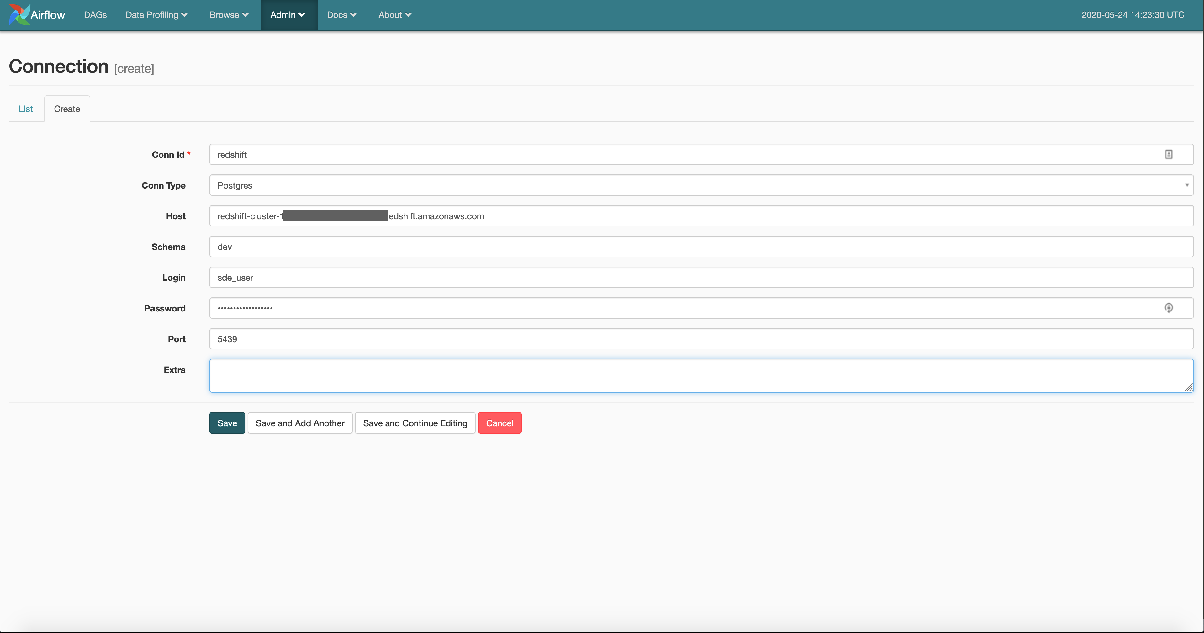
We have the movie review and user purchase data cleaned and ready in the staging S3 location. We need to enable airflow to connect to our redshift database. To do this we go to Airflow UI -> Admin -> Connections and click on the Create tab.
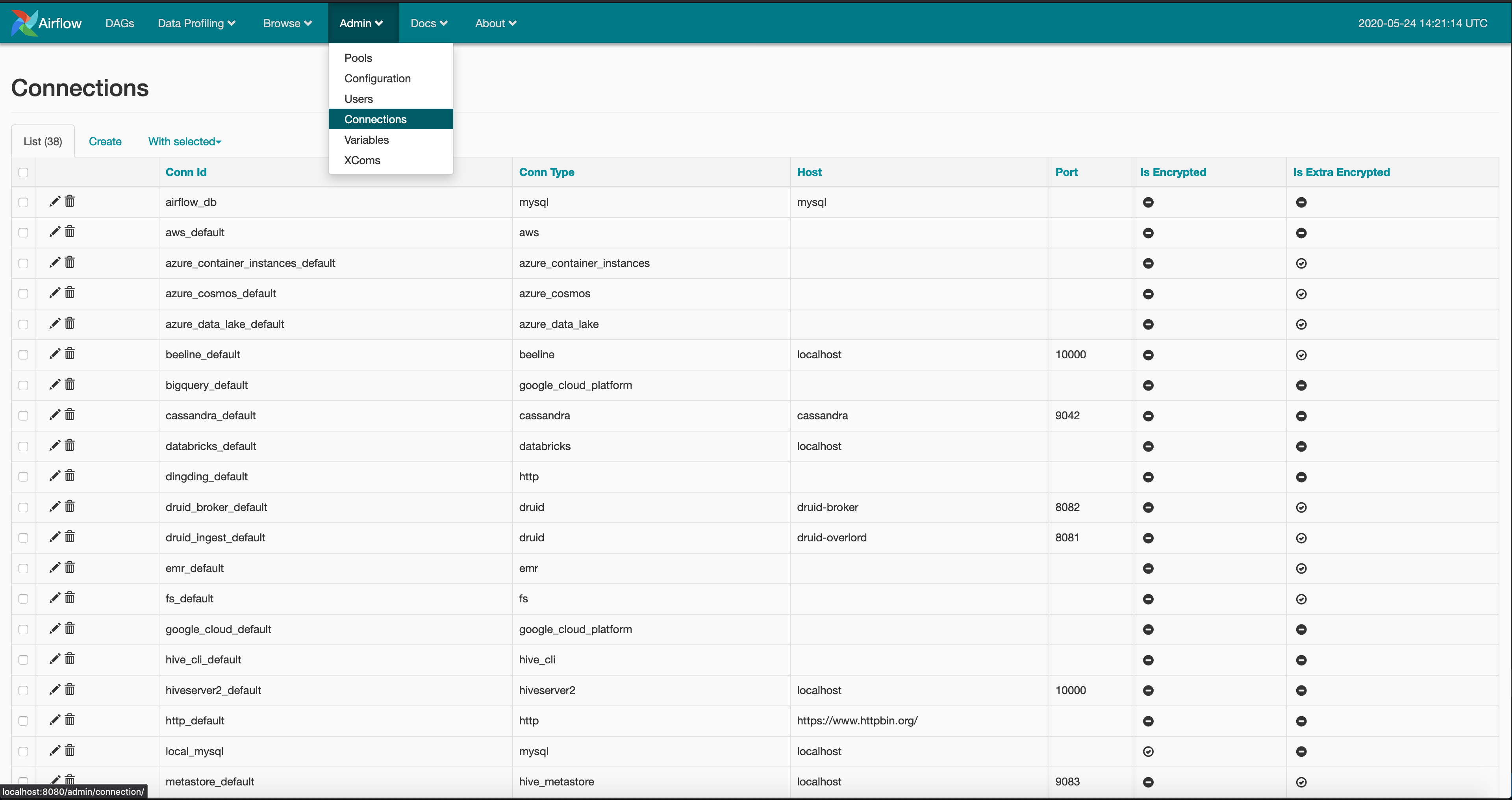
And create a postgres type connection with the name redshift, using your redshift credentials. These define how your airflow instance will connect to your redshift cluster.
Once we have the connection established, we need to let the user_purchase_staging table know that a new partition has been added. We can do that on our DAG as shown below.
# existing imports
from airflow.hooks.postgres_hook import PostgresHook
import psycopg2

# existing helper function(s)
def run_redshift_external_query(qry):
    rs_hook = PostgresHook(postgres_conn_id='redshift')
    rs_conn = rs_hook.get_conn()
    rs_conn.set_isolation_level(psycopg2.extensions.ISOLATION_LEVEL_AUTOCOMMIT)
    rs_cursor = rs_conn.cursor()
    rs_cursor.execute(qry)
    rs_cursor.close()
    rs_conn.commit()

# existing tasks
user_purchase_to_rs_stage = PythonOperator(
    dag=dag,
    task_id='user_purchase_to_rs_stage',
    python_callable=run_redshift_external_query,
    op_kwargs={
        'qry': "alter table spectrum.user_purchase_staging add partition(insert_date='{{ ds }}') \
            location 's3://<your-bucket>/user_purchase/stage/{{ ds }}'",
    },
)

# existing task dependency def
remove_local_user_purchase_file >> user_purchase_to_rs_stage
This is a tricky one. If we are using normal redshift we can use the PostgresOperator to execute queries, since Redshift is based on Postgres. But because we are working with external tables
we cannot use it, instead we have to open a postgres connection using PostgresHook and we have to set the appropriate isolation level. You can create your own operator to handle this, but since this is an example we are not creating a separate operator. The query passed as qry to the python function is an alter statement letting the user_purchase_staging table know that a new partition has been added at s3://<your-bucket>/user_purchase/stage/yyyy-mm-dd. The final task is to load data into our user_behavior_metric table. Let’s write a templated query to do this at beginner_de_project/dags/scripts/sql/get_user_behavior_metrics.sql
INSERT INTO public.user_behavior_metric
(customerid,
amount_spent,
review_score,
review_count,
insert_date)

SELECT ups.customerid,
cast(sum( ups.Quantity * ups.UnitPrice) as decimal(18, 5)) as amount_spent,
sum(mrcs.positive_review) as review_score, count(mrcs.cid) as review_count,
'{{ ds }}'
FROM spectrum.user_purchase_staging ups
JOIN (select cid, case when positive_review is True then 1 else 0 end as positive_review from spectrum.movie_review_clean_stage) mrcs
ON ups.customerid = mrcs.cid
WHERE ups.insert_date = '{{ ds }}'
GROUP BY ups.customerid;
We are getting customer level metrics and loading them into a user_behavior_metric table. Add this as a task to our DAG as shown below
# existing config
get_user_behaviour = 'scripts/sql/get_user_behavior_metrics.sql'

# existing tasks
get_user_behaviour = PostgresOperator(
    dag=dag,
    task_id='get_user_behaviour',
    sql=get_user_behaviour,
    postgres_conn_id='redshift'
)

pg_unload >> user_purchase_to_s3_stage >> remove_local_user_purchase_file >> user_purchase_to_rs_stage
[movie_review_to_s3_stage, move_emr_script_to_s3] >> add_emr_steps >> clean_movie_review_data
[user_purchase_to_rs_stage, clean_movie_review_data] >> get_user_behaviour >> end_of_data_pipeline
Your airflow DAG should look like this
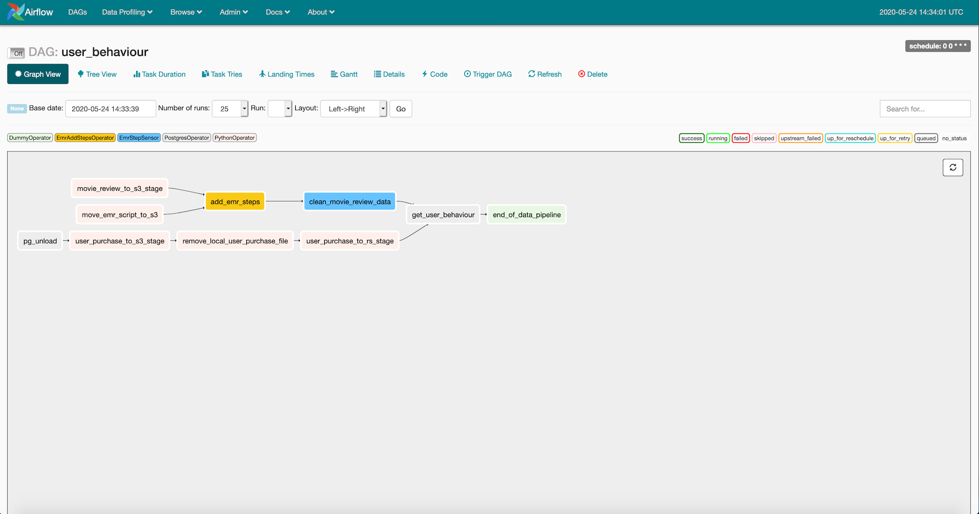
Congratulations you have your data pipeline setup. Verify that it completes successfully from the Airflow UI and using pgcli connect to your redshift instance and run the query
select * from public.user_behavior_metric limit 10;
you should see the data with insert_date 2010-12-01 for the first run. Do not forget to switch off you Redshift cluster and EMR cluster. You can spin down your docker containers using
docker-compose -f docker-compose-LocalExecutor.yml down
docker-compose -f docker-compose-LocalExecutor.yml up -d
Monitoring ETL
Before you start running the DAG it would be good to understand how to monitor them as they are long running processes consuming a lot of memory.
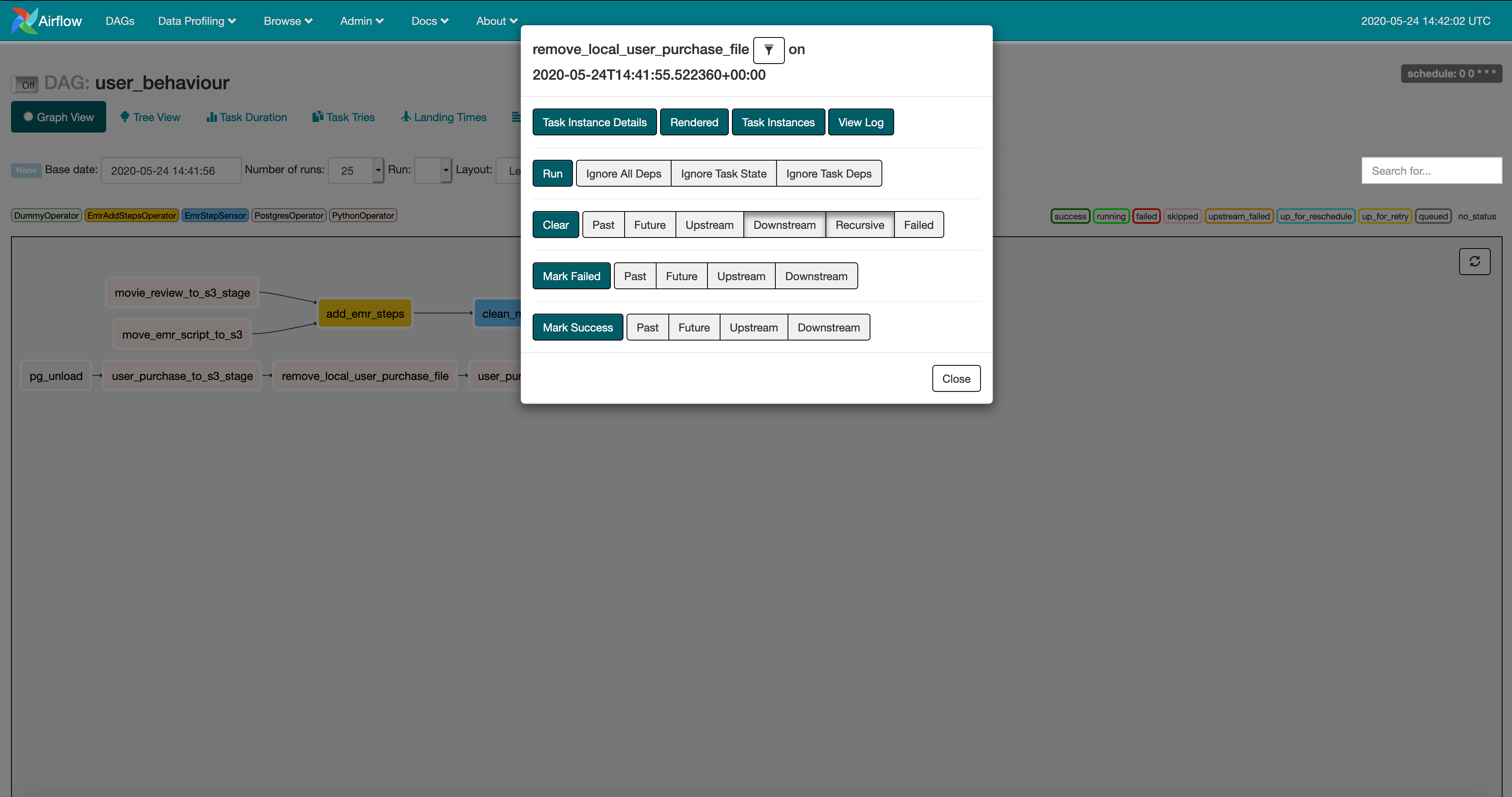
-
Airflow UI, in the airflow UI you can monitor the status, logs, task details(note that some of these are only visible after the DAG is started)
-
Since we are running a Spark application on an EMR cluster we can monitor the Spark job status using the Spark UI that you can find on your emr page.
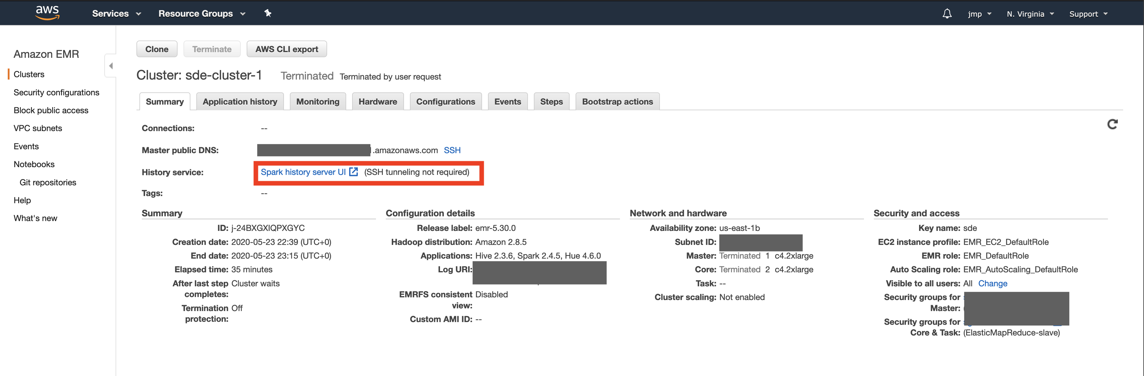
-
The Spark UI provides spark task level details
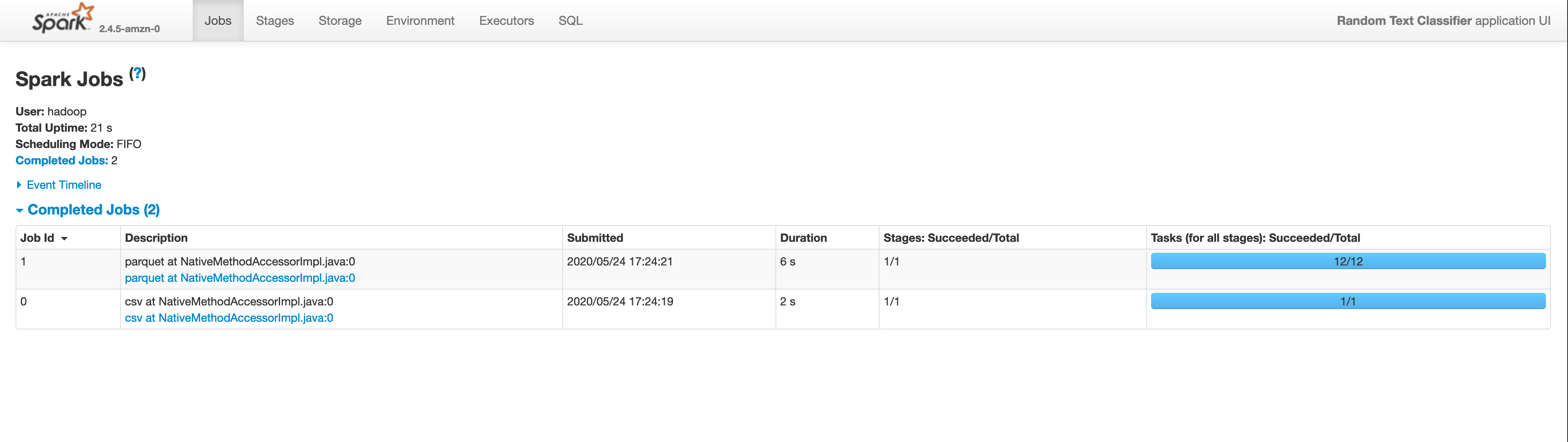
-
Redshift has its own query monitoring capabilities ref .
Design Review
In our data pipeline there are some obvious issues let’s review them
-
We are pulling data from an OLTP database, this is usually a bad idea since OLTP databases are meant to be used for app level transactions. And depending on the size of this query it can significantly slow down the other queries on this OLTP database. In cases like these we should use some sort of trickle down approach such as using Debezium . And also, If we want to run multiple DAGs in parallel we cannot since the temp file location is not name spaced by date. i.e we can’t simultaneously run the
remove_local_user_purchase_filefor a DAG run andpg_unloadfor its next DAG run, since they might run into a race condition when writing and reading the same named file. This can be prevented by saving the file in a location such as../yyyy-mm-dd-hh-mm/temp_file.csv. -
Here we are overwriting the same data in load and stage areas. This means that our movie review stage table only contains the latest days data. This is extremely dangerous. If we want to make a backfill for specific dates(for whatever business reasons), it would be very difficult since we will have to go back to vendor to get that data. If we have stored the data in folders partitioned by time(similar to the way we store
user_purchase_staging) it would have been a simple backfill in Airflow.
Common Scenarios
When running a batch data pipeline on Airflow you face some common scenarios they are
-
backfill, its when the company wants to make a historical change to the way data is processed, e.g they might say on May 24th 2020, that they want all data from July 1st, 2019 to be filter to have
quantity > 5as opposed to the> 2filter we had. In this scenario it is very beneficial to use a date based, mature system like airflow because it has inbuilt capabilities for this exact scenario. ref -
The
DAGis not getting started, this is a commonly from other engineers. It is mostly due to theparallelismordag_concurrencyor wrongly set pool size -
Not designing idempotent and independent tasks. This will cause overwrites or lead to deleting crucial data. Similar to the issue of movie review we saw in the design review above.
-
Not reading Common pitfalls
Next Steps
-
Create a data quality check task after the
get_user_behaviourtask to check for data presence using count. -
Understand what
wait_for_downstreamanddepends_on_pastoptions we set are. -
Try to recreate this
DAG, but scheduled hourly instead of daily. What would need to change? what are the pros and cons of this? -
Understand Airflow is running on UTC time, and what this means for how you filter the user purchase data. Most companies store data at UTC and translate to local time at the application layer.
-
Try to make DAG fully parallel and run backfill where DAG’s are run in parallel, research
max_active_runsparameter in your code. -
If you data size increases by 10x, 100x, 1000x reason about if/how your data pipeline will handle the load, will it just take more time or straight up fail?
-
Go over
docker-compose-*.ymlfiles in the repo to understand the components involved in airflow setup, and the volume mounts we have. -
If you have a new idea you would like to see, or report an issue then do a PR or create an issue at https://github.com/josephmachado/beginner_de_project
-
Using a OLAP database (AWS Redshift in our case) is very different from a traditional OLAP database. Make sure to read redshift best practices and understand what can be done to make our design scalable and performant.
Conclusion
Initially the plan was to build a data pipeline with both batch and streaming pipelines. But that got too big for one blog post. So I decided to split them into 2 separate ones. The next post in this series will be a streaming data processing pipeline. Let me know in the comments section below if you would like to see anything specific.
Hope this article gives you a good idea of the nature and complexity of batch data processing. Let me know if you have any questions or comments in the comment section below. Good Luck.