3 Data Storage Techniques Every Data Engineer Should Know

Most Data Processing Costs Are Due to Full Table Scans

In a data warehouse, data is read far more often than it is written into. If you:

See data costs skyrocket as vendors charge based on the amount of data scanned & the compute to process it

Find yourself getting stuck when an interviewer asks, “How would you optimize this pipeline?” in design interviews

See BI tools/dashboards failing due to queries taking a really long time to run

This post is for you.

You can create data that is cheap and fast to query. We will see how you can do that in this post.

By the end of this post, you will have

• Data storage rule-of-thumb for analytical tables
• A way to 80% improvement in query cost & speed

To follow along with code

1. Clone and start Spark containers as shown here.
2. Open storage_patterns.ipynb and run the setup.

Only Read the Data You Want to Process

Most analytical queries include the same filters/joins/group by columns.

Store data in a way that enables the data processing system to only read the data needed by those queries.

Follow these rules of thumb and see your queries fly

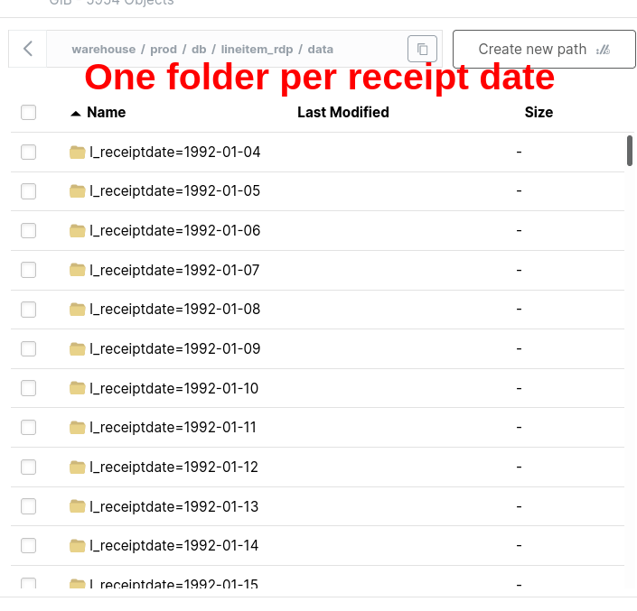
Partition Fact Table by date(created_at), as It’s Often Filtered or Grouped by This Column

NoteRule of thumb

• Partition your fact table on date(created_at) or hour(created_at) if data is very large.

• Partition snapshot dimension on loaded_at. Read it as shown below.

  select * 
  from snapshot_dimension 
  where loaded_at = (select max(loaded_at) from snapshot_dimension)

• Do not partition SCD2 table.

Let’s partition a table.

# create a partitioned table
spark\
.read\
.table("lineitem")\
.writeTo("lineitem_rdp")\
.partitionedBy("l_receiptdate")\
.createOrReplace()

Partitioned Data

We will see that the filter on a partitioned table does not have in-memory filtering.

The process of selecting only the partition we need at the read level is called Partition Pruning.

# PARTITION PRUNING = Only read the necessary partition
# No in-memory filtering
spark\
.read\
.table("lineitem_rdp")\
.where(F.col("l_receiptdate") == "1992-01-05")\
.explain()

== Physical Plan ==
*(1) ColumnarToRow
+- BatchScan demo.prod.db.lineitem_rdp[l_orderkey#80, l_partkey#81, l_suppkey#82, l_linenumber#83, l_quantity#84, l_extendedprice#85, l_discount#86, l_tax#87, l_returnflag#88, l_linestatus#89, l_shipdate#90, l_commitdate#91, l_receiptdate#92, l_shipinstruct#93, l_shipmode#94, l_comment#95] demo.prod.db.lineitem_rdp (branch=null) [filters=l_receiptdate IS NOT NULL, l_receiptdate = 8039, groupedBy=] RuntimeFilters: []

The filter l_receiptdate = 8039 indicates the date in epoch days and is done at the storage level.

Let’s compare this with a query on a table without partitioning.

Query Performance

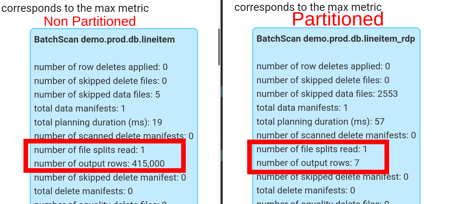
We can see how partition pruning makes queries more efficient by reading only the necessary data.

Use multi-column partition only when there is a measurable improvement across uses. Premature optimization can make queries slower by making the file size per partition too small.

Ensure your tech takes advantage of partitions. Older systems (Hive) have limitations around partition order, transformation-based partition, etc.

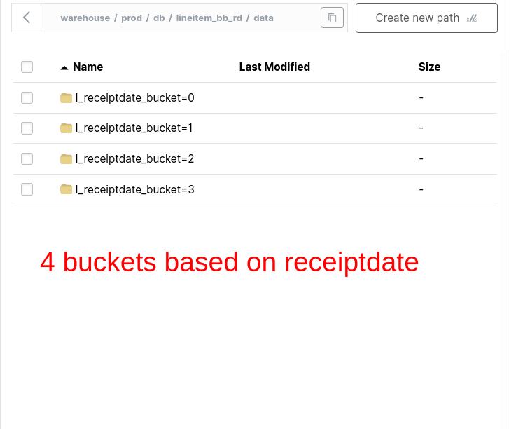
Bucket Fact Table on the ID Commonly Used in Join/Group By

NoteRule of thumb

• Bucket on high-cardinality columns (columns with lots of unique values or a numerical range of values)

• Bucket fact table on column that’s used frequently to join another fact table or in group by

• Only bucket snapshot dimension if it is a very large (approx > 5 million rows) by its natural id or common join id

Let’s bucket a table.

# Create a bucketed table, with the bucketing based on the group by column
from pyspark.sql import functions as F
spark.read.table("lineitem")\
.writeTo("lineitem_bb_rd") \
.partitionedBy(  
    F.partitioning.bucket(4, "l_receiptdate")
).createOrReplace()

Bucketing is a type of partitioning.

Bucketed Lineitem

Bucketing helps avoid exchanges.

BUCKETING = NO Exchange
# settings to ensure Spark + Iceberg can leverage the underlying data layout
spark.conf.set(‘spark.sql.sources.v2.bucketing.enabled’,‘true’)
spark.conf.set(‘spark.sql.iceberg.planning.preserve-data-grouping’,‘true’)

spark\
.sql("""
SELECT l_receiptdate
, sum(l_quantity) as total_quantity
FROM lineitem_bb_rd
GROUP BY l_receiptdate
""")\
.explain()

#| code-overflow: wrap
== Physical Plan ==
AdaptiveSparkPlan isFinalPlan=false
+- HashAggregate(keys=[l_receiptdate#196], functions=[sum(l_quantity#188)])
   +- HashAggregate(keys=[l_receiptdate#196], functions=[partial_sum(l_quantity#188)])
      +- BatchScan demo.prod.db.lineitem_bb_rd[l_quantity#188, l_receiptdate#196] demo.prod.db.lineitem_bb_rd (branch=null) [filters=, groupedBy=l_receiptdate_bucket] RuntimeFilters: []

We can see that there is no exchange. Because the l_receiptdate data is colocated and will be read by a single executor for computing aggregates.

Caution

Partitioning takes precedence; use bucketing only if it provides measurable gains in joins/group bys.

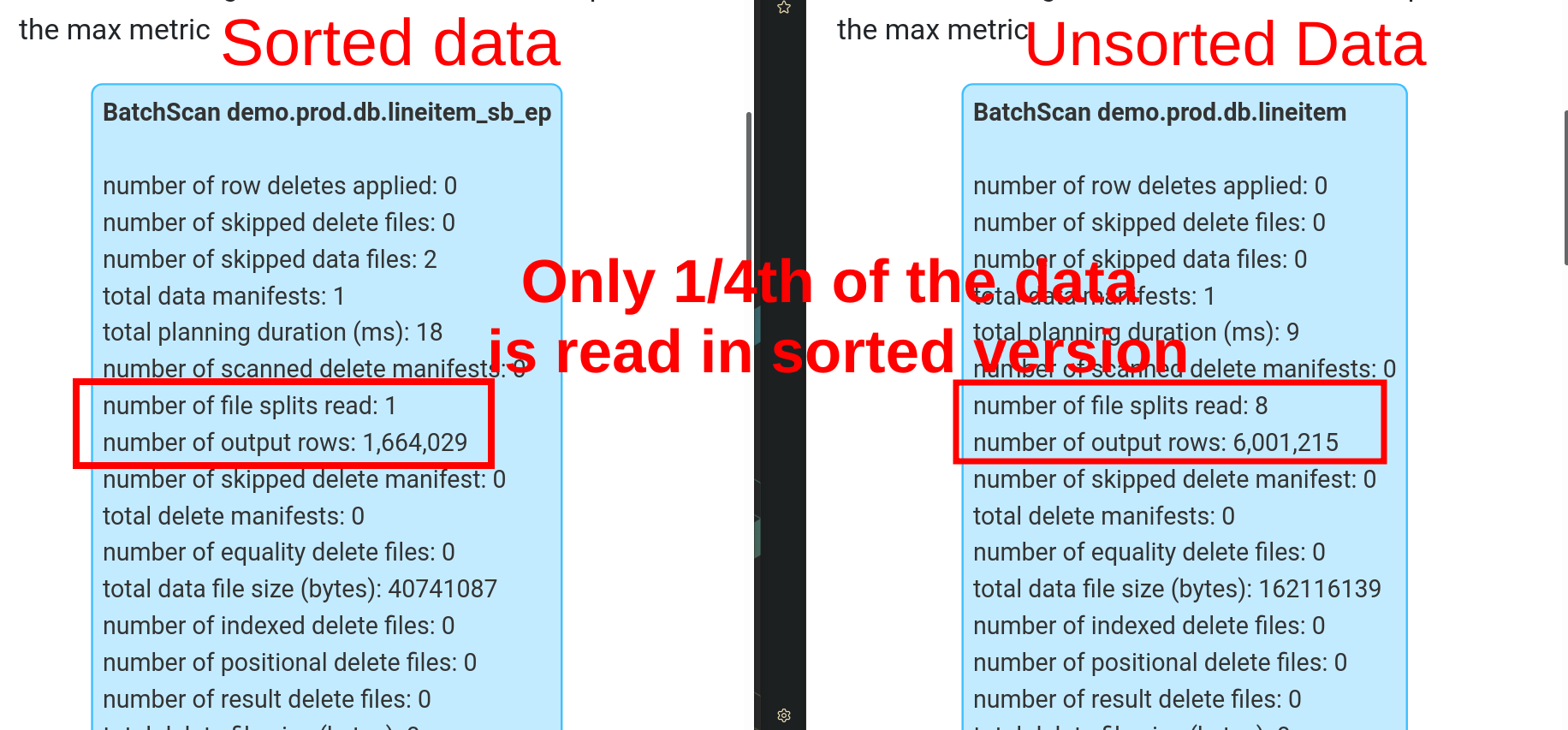
Sorting Makes Filter Pushdowns Effective by Reading Only the Necessary row_group

• Filter pushdown is when a data processing engine uses metadata to only read the necessary data chunk on disk.

NoteRule of thumb

• Sort fact data on created_at timestamp, if there are no commonly filtered by numerical column.

Let’s sort our fact table.

# Create Sorted Table
spark.read.table("lineitem")\
.sort("l_extendedprice")\
.coalesce(3)\
.writeTo("lineitem_sb_ep")\
.createOrReplace()

Let’s compare how the filter works on a sorted table.

# SORTING = Smaller data read into Spark Memory
spark.sql("""
select *
from lineitem_sb_ep
where l_extendedprice between 3000 and 10000
""")\
.write\
.csv(f"./{chapter_name}/lineitem_0rd", mode = 'overwrite')

Sorted v Non Sorted Filter

Choosing an Appropriate Storage Pattern Is 80% of Pipeline Optimization

We saw why to

1. Partition fact table by date(created_at)
2. Bucket fact table on commonly used join/group by id
3. Sort data to only read the necessary data chunks

Using these techniques will cover 80% of your optimization needs.

Start simple with these rules of thumb.

Only add more complexity if you see significant benefits. Comment below and let me know how you optimize your pipelines.

Read These

1. Snapshot & SCD2 Dimension
2. SQL Optimizations
3. Storage Partition Join